Date Archives

May 2023

Navigating the Path: Exploring the Pros and Cons of Regulating AI

Navigating the Path: Exploring the Pros and Cons of Regulating AI

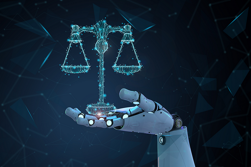
Artificial Intelligence (AI) has evolved at an unprecedented pace, permeating various aspects of our lives. From autonomous vehicles to virtual assistants and complex algorithms, AI has become deeply intertwined with our daily routines. However, as this powerful technology continues to advance, questions regarding the need for regulation have emerged. In this article, we will delve into the multifaceted topic of regulating AI, examining both the benefits and challenges that accompany such measures.

The Potential Benefits of Regulating AI

  1. Ethical Framework: One of the primary motivations behind regulating AI is to establish an ethical framework that guides its development and deployment. AI systems possess the ability to make autonomous decisions that have a profound impact on individuals and society as a whole. By implementing regulations, we can ensure that AI is developed and utilized in a manner that aligns with our shared values and ethical principles.
  2. Safety and Security: AI-powered systems can wield immense power, and if left unchecked, they could potentially pose risks to safety and security. Regulating AI can promote the implementation of safeguards and standards that mitigate potential threats. This includes addressing issues such as bias in AI algorithms, ensuring data privacy, and preventing the malicious use of AI technologies.
  3. Transparency and Accountability: AI algorithms can sometimes operate as “black boxes,” making it challenging to comprehend the decision-making processes behind their outputs. By regulating AI, we can encourage transparency and accountability, making it easier to understand how these systems arrive at their conclusions. This fosters trust among users and allows for the identification and rectification of potential biases or errors.

The Challenges of Regulating AI

  1. Innovation and Progress: Overregulation can stifle innovation by burdening AI developers with excessive constraints. Striking the right balance between regulation and fostering innovation is crucial. It is important to avoid impeding the advancement of AI technology, as it holds tremendous potential for addressing complex societal challenges and driving economic growth.
  2. Global Consensus: AI operates on a global scale, and establishing consistent regulations across different countries can be challenging. Varying legal frameworks and cultural differences make it difficult to create unified rules governing AI technology. International collaboration and cooperation will be necessary to address these challenges effectively.
  3. Adaptability and Agility: Technology evolves rapidly, often outpacing the ability to create comprehensive regulations. Prescriptive and rigid regulations may struggle to keep up with the dynamic nature of AI, potentially rendering them obsolete or inadequate. Crafting regulatory frameworks that can adapt to evolving technologies while remaining effective is a complex task.

Balancing Act: A Collaborative Approach

Regulating AI requires a balanced approach that considers the potential benefits and challenges involved. Rather than viewing regulation as a restrictive force, it should be seen as an enabler, fostering responsible and beneficial use of AI technology.

To achieve this, collaboration between various stakeholders is crucial. Governments, industry leaders, AI developers, researchers, and ethicists need to engage in thoughtful dialogue to craft regulations that strike the right balance. This collaborative approach ensures that regulations are informed by technical expertise, societal values, and the concerns of all relevant parties.

Moreover, a continuous feedback loop is necessary to refine regulations as the technology progresses. Regular evaluations, audits, and adaptive frameworks can help ensure that regulations remain effective and up to date.

Regulating AI presents both opportunities and challenges. Establishing a framework that encourages innovation, while safeguarding ethics, safety, and transparency, is key. By engaging in a collaborative approach and embracing continuous learning and adaptation, we can harness the potential of AI while ensuring that it aligns with our shared values. With responsible regulation, we can navigate the path of AI development and deployment, shaping a future where AI serves as a force for positive change.\

What do you think?

What are your thoughts on Regulating AI?

Preparing Apache and NGINX logs for use with Machine Learning

Preparing Apache and NGINX logs for use with Machine Learning

Preparing Apache Logs for Machine Learning

Apache logs often come in a standard format known as the Combined Log Format. It includes client IP, date, request method, status code, user agent, and other information. To use this data with machine learning algorithms, we need to transform it into numerical form.

Here’s a simple Python script using the pandas and apachelog libraries to parse Apache logs:

Step 1: Import Necessary Libraries

import pandas as pd
import apachelog

Step 2: Define Log Format

# This is the format of the Apache combined logs
format = r'%h %l %u %t \"%r\" %>s %b \"%{Referer}i\" \"%{User-Agent}i\"'
p = apachelog.parser(format)

Step 3: Parse the Log File

def parse_log(file):
    data = []
    for line in open(file):
        try:
            data.append(p.parse(line))
        except:
            pass
    return pd.DataFrame(data, columns=['ip', 'client', 'user', 'datetime', 'request', 'status', 'size', 'referer', 'user_agent'])

df = parse_log('access.log')

Now you can add a feature extraction step to convert these categorical features into numerical ones, for example, using one-hot encoding or converting IP addresses into numerical values.

Preparing Nginx Logs for Machine Learning

The process is similar to the one we followed for Apache logs. Nginx logs usually come in a very similar format to Apache’s Combined Log Format.

Step 1: Import Necessary Libraries

import pandas as pd
import pynginxlog

Step 2: Define Log Format

# This is the standard Nginx log format
format = r'$remote_addr - $remote_user [$time_local] "$request" $status $body_bytes_sent "$http_referer" "$http_user_agent"'
p = pynginxlog.NginxParser(format)

Step 3: Parse the Log File

def parse_log(file):
    data = []
    for line in open(file):
        try:
            data.append(p.parse(line))
        except:
            pass
    return pd.DataFrame(data, columns=['ip', 'client', 'user', 'datetime', 'request', 'status', 'size', 'referer', 'user_agent'])

df = parse_log('access.log')

Again, you will need to convert these categorical features into numerical ones before feeding them into the machine learning model.

Anomaly Detection in System Logs using Machine Learning (scikit-learn, pandas)

Anomaly Detection in System Logs using Machine Learning (scikit-learn, pandas)

In this tutorial, we will show you how to use machine learning to detect unusual behavior in system logs. These anomalies could signal a security threat or system malfunction. We’ll use Python, and more specifically, the Scikit-learn library, which is a popular library for machine learning in Python.

For simplicity, we’ll assume that we have a dataset of logs where each log message has been transformed into a numerical representation (feature extraction), which is a requirement for most machine learning algorithms.

Requirements:

  • Python 3.7+
  • Scikit-learn
  • Pandas

Step 1: Import Necessary Libraries

We begin by importing the necessary Python libraries.

import pandas as pd
from sklearn.ensemble import IsolationForest
from sklearn.preprocessing import StandardScaler

Step 2: Load and Preprocess the Data

We assume that our log data is stored in a CSV file, where each row represents a log message, and each column represents a feature of the log message.

# Load the data
data = pd.read_csv('logs.csv')

# Normalize the feature data
scaler = StandardScaler()
data_scaled = scaler.fit_transform(data)

Step 3: Train the Anomaly Detection Model

We will use the Isolation Forest algorithm, which is an unsupervised learning algorithm that is particularly good at anomaly detection.

# Train the model
model = IsolationForest(contamination=0.01)  # The contamination parameter is used to control the proportion of outliers in the dataset
model.fit(data_scaled)

Step 4: Detect Anomalies

Now we can use our trained model to detect anomalies in our data.

# Predict the anomalies in the data
anomalies = model.predict(data_scaled)

# Find the index of anomalies
anomaly_index = where(anomalies==-1)
# Print the anomaly data
print("Anomaly Data: ", data.iloc[anomaly_index])

With this code, we can detect anomalies in our log data. You might need to adjust the contamination parameter depending on your specific use case. Lower values will make the model less sensitive to anomalies, while higher values will make it more sensitive.

Also, keep in mind that this is a simplified example. Real log data might be more complex and require more sophisticated feature extraction techniques.

Step 5: Evaluate the Model

Evaluating an unsupervised machine learning model can be challenging as we usually do not have labeled data. However, if we do have labeled data, we can evaluate the model by calculating the F1 score, precision, and recall.

from sklearn.metrics import classification_report

# Assuming that "labels" is our ground truth
print(classification_report(labels, anomalies))

That’s it! You have now created a model that can detect anomalies in system logs. You can integrate this model into your DevOps workflow to automatically identify potential issues in your systems.

Concurrency and Goroutines: Understanding Concurrency and Goroutines in Go

Concurrency and Goroutines: Understanding Concurrency and Goroutines in Go

Concurrency is an essential concept in modern programming, allowing multiple tasks to run concurrently and efficiently utilize system resources. Go, a statically typed programming language developed by Google, provides built-in support for concurrency through Goroutines and channels. In this tutorial, we will explore how to leverage Goroutines and manage concurrency using GoLand, a popular integrated development environment (IDE) for Go.

1. Introduction to Concurrency in Go

Concurrency is the ability of a program to perform multiple tasks simultaneously, making efficient use of system resources such as CPU cores. Go introduces concurrency as a core language feature, enabling developers to write concurrent programs easily and efficiently.

Go achieves concurrency through Goroutines, which are lightweight concurrent execution units, and channels, which provide synchronization and communication between Goroutines.

2. Goroutines: Lightweight Concurrent Execution Units

A Goroutine is a function that can be executed concurrently with other Goroutines. They are lightweight and have a smaller memory footprint compared to operating system threads. Goroutines are managed by the Go runtime, allowing efficient scheduling and execution of concurrent tasks.

The go keyword is used to start a new Goroutine. When a Goroutine is created, it runs concurrently with the main Goroutine or other Goroutines, allowing parallel execution.

3. Creating and Running Goroutines

Let’s dive into some code examples to see how Goroutines are created and run in Go. Assume we have a function process() that performs some time-consuming task.

func process() {
    // Perform some time-consuming task
}

To execute this function concurrently using a Goroutine, we can use the go keyword:

go process()

The go keyword launches a new Goroutine, and process() will start executing concurrently. The main Goroutine and the newly created Goroutine will run independently.

4. Synchronization with Channels

Channels in Go provide a mechanism for Goroutines to communicate and synchronize their execution. A channel is a typed conduit that allows sending and receiving values between Goroutines.

Let’s consider an example where we have two Goroutines: a producer and a consumer. The producer generates some data and sends it to the consumer using a channel.

func producer(ch chan<- int) {
    for i := 0; i < 5; i++ {
        ch <- i // Send data to the channel
    }
    close(ch) // Close the channel to signal the end of data
}

func consumer(ch <-chan int) {
    for num := range ch {
        fmt.Println(num) // Print the received data
    }
}

In this example, the producer Goroutine sends integers to the channel ch, and the consumer Goroutine receives and prints them. The ch channel is created with the type chan int, indicating it can only send or receive integers.

To execute the producer and consumer concurrently, we can create a channel and launch the Goroutines using the go keyword:

ch := make(chan int)
go producer(ch)
go consumer(ch)

The producer Goroutine sends data to the channel, and the consumer Goroutine receives and prints it. This synchronization ensures that the consumer only processes data when it is available.

5. GoLand’s Tools for Managing Goroutines

GoLand, an IDE developed by JetBrains, provides powerful tools to manage Goroutines and visualize concurrent execution.

Debugging Goroutines

GoLand offers a rich set of debugging features for Goroutines. You can set breakpoints, inspect variables, and step through Goroutines to identify and fix issues in concurrent code.

To debug Goroutines in GoLand, follow these steps:

  1. Set a breakpoint in the code where you want to start debugging.
  2. Run the program in debug mode by clicking on the “Debug” button or using the corresponding keyboard shortcut.
  3. When the breakpoint is hit, the program execution will pause.
  4. Use the debugging toolbar to step through the code, inspect variables, and analyze Goroutine behavior.

Goroutine Visualization

Understanding the flow of Goroutines and how they interact can be challenging in complex concurrent programs. GoLand provides a visual Goroutine tool that helps you analyze the Goroutine execution flow.

To visualize Goroutines in GoLand, follow these steps:

  1. Run your program in debug mode.
  2. Open the “Goroutines” tab in the Debug tool window.
  3. The “Goroutines” tab displays a list of active Goroutines and their current state.
  4. You can see the Goroutine stack traces, examine their state, and navigate through them to understand the execution flow.

Profiling Goroutines

Profiling is crucial for optimizing performance in concurrent programs. GoLand integrates with Go’s profiling tools to help you analyze Goroutine behavior and identify bottlenecks.

To profile Goroutines in GoLand, follow these steps:

  1. Open the “Run” menu and select “Profile”.
  2. Choose the profiling type you want, such as CPU profiling or memory profiling.
  3. Run your program with the selected profiling configuration.
  4. GoLand will collect profiling data and present it in an interactive UI.
  5. Analyze the Goroutine-specific profiling results to identify performance issues and optimize your code.

Concurrency and Goroutines are fundamental to writing efficient and scalable programs in Go. With GoLand’s powerful tools for managing Goroutines, you can debug, visualize, and profile concurrent code effectively.

In this tutorial, we covered the basics of concurrency and Goroutines in Go, including creating and running Goroutines, synchronizing with channels, and leveraging GoLand’s tools for managing Goroutines. Armed with this knowledge, you can confidently write concurrent programs in Go and utilize GoLand’s features to enhance your development workflow.

Remember, concurrency can be complex, so it’s important to understand the principles and best practices to write correct and efficient concurrent code. Keep exploring the vast possibilities of Goroutines and Go’s concurrency features to build robust and highly performant applications.

Demand Clustering and Segmentation with Machine Learning in Logistics (Kmeans, scikit-learn, matplotlib)

Demand Clustering and Segmentation with Machine Learning in Logistics (Kmeans, scikit-learn, matplotlib)

In the field of logistics, understanding and predicting customer demand patterns is crucial for optimizing supply chain operations. By employing machine learning techniques, we can cluster and segment demand data to uncover valuable insights and make informed decisions. In this tutorial, we will explore how to perform demand clustering and segmentation using Python and popular machine learning libraries.

Prereqs

To follow along with this tutorial, you’ll need:

  • Python 3.x installed on your system
  • The following Python libraries: pandas, numpy, scikit-learn, matplotlib

You can install the required libraries using pip:

pip install pandas numpy scikit-learn matplotlib

Step 1: Data Preparation

The first step is to gather and prepare the demand data for analysis. This typically involves loading the data into a pandas DataFrame and performing any necessary preprocessing steps such as handling missing values or normalizing the data. For this tutorial, we’ll assume you have a CSV file containing demand data with the following columns: dateproduct_idquantity.

Let’s start by importing the necessary libraries and loading the data:

import pandas as pd

# Load the demand data from CSV
demand_data = pd.read_csv('demand_data.csv')

Next, we can examine the data and perform any necessary preprocessing steps. This might include handling missing values, converting data types, or normalizing the data. Preprocessing steps will vary depending on the specific dataset and requirements of your analysis.

Step 2: Feature Engineering

To apply machine learning algorithms, we need to extract relevant features from the demand data. In this tutorial, we’ll use the following features: product_idquantity, and date (as a temporal feature). We’ll transform the date column into separate features such as year, month, day, and day of the week. Additionally, we can include other domain-specific features if available, such as product category or customer segment.

Let’s create a function to perform feature engineering:

from datetime import datetime

def engineer_features(data):
    # Convert date column to datetime
    data['date'] = pd.to_datetime(data['date'])
    # Extract year, month, day, and day of the week
    data['year'] = data['date'].dt.year
    data['month'] = data['date'].dt.month
    data['day'] = data['date'].dt.day
    data['day_of_week'] = data['date'].dt.dayofweek
    # Include other relevant features if available
    return data
# Apply feature engineering
demand_data = engineer_features(demand_data)

Step 3: Demand Clustering

Now that we have prepared our data and engineered the necessary features, we can proceed with demand clustering. Clustering is an unsupervised learning technique that groups similar instances together based on their features. In our case, we want to cluster demand patterns based on the extracted features.

For this tutorial, we’ll use the popular K-means clustering algorithm. Let’s import the required libraries and perform the clustering:

from sklearn.cluster import KMeans

# Select relevant features for clustering
features = ['quantity', 'year', 'month', 'day', 'day_of_week']
# Perform clustering
kmeans = KMeans(n_clusters=3)
clusters = kmeans.fit_predict(demand_data[features])

In the code above, we selected the features to be used for clustering (quantityyearmonthdayday_of_week) and specified the number of clusters to be 3. You can adjust these parameters according to your specific use case.

Step 4: Demand Segmentation

Once we have performed demand clustering, we can further segment the clusters to gain deeper insights into different customer demand patterns. Segmentation helps us understand distinct groups within each cluster, allowing us to tailor our logistics strategies accordingly.

In this tutorial, we’ll use the K-means clustering results to perform segmentation. We’ll calculate the centroid of each cluster and assign demand data points to the nearest centroid. This will help us identify which products or time periods belong to each segment within a cluster.

Let’s continue with the code:

# Add cluster labels to the demand data
demand_data['cluster'] = clusters

# Calculate the centroid of each cluster
cluster_centroids = pd.DataFrame(kmeans.cluster_centers_, columns=features)
# Segment the demand data based on cluster centroids
segment_labels = kmeans.predict(cluster_centroids)
demand_data['segment'] = demand_data['cluster'].apply(lambda x: segment_labels[x])

In the code above, we added the cluster labels to the demand data. Then, we calculated the centroid of each cluster using the cluster_centers_ attribute of the K-means model. Next, we predicted the segment labels for each cluster centroid using the predict method. Finally, we assigned the segment labels to the demand data based on their corresponding cluster.

Step 5: Visualizing Clusters and Segments

To better understand the clustering and segmentation results, it’s helpful to visualize them. We can plot the clusters and segments on different charts to observe patterns and identify differences between them.

Let’s create a scatter plot to visualize the clusters:

import matplotlib.pyplot as plt

# Plot clusters
plt.scatter(demand_data['quantity'], demand_data['year'], c=demand_data['cluster'])
plt.xlabel('Quantity')
plt.ylabel('Year')
plt.title('Demand Clusters')
plt.show()

Similarly, we can create a bar chart to visualize the segments:

segment_counts = demand_data['segment'].value_counts()

# Plot segments
plt.bar(segment_counts.index, segment_counts.values)
plt.xlabel('Segment')
plt.ylabel('Count')
plt.title('Demand Segments')
plt.show()

By visualizing the clusters and segments, we can gain insights into the distinct demand patterns within our data. This information can be used to make data-driven decisions and optimize logistics operations accordingly.

In this tutorial, we explored how to perform demand clustering and segmentation using machine learning in logistics. We learned how to prepare the data, engineer relevant features, apply clustering algorithms, and segment the results. Additionally, we visualized the clusters and segments to gain insights into the demand patterns.

By employing these techniques, logistics professionals can effectively analyze customer demand, uncover hidden patterns, and optimize their supply chain operations for improved efficiency and customer satisfaction.

Remember, demand clustering and segmentation is just one aspect of utilizing machine learning in logistics. There are many other techniques and models that can be applied to tackle different challenges in the field. So feel free to explore further and expand your knowledge!

Happy coding!

Predicting Delivery Time and Estimating Shipment Delays with Machine Learning (Supply Chain and Logistics Series)

Predicting Delivery Time and Estimating Shipment Delays with Machine Learning (Supply Chain and Logistics Series)

In today’s fast-paced world, efficient delivery and logistics are crucial for businesses. Predicting delivery times accurately and estimating shipment delays can help companies streamline their operations, optimize resources, and provide better customer service. Machine learning techniques can be employed to analyze historical data and build predictive models that can forecast delivery times and identify potential delays. In this tutorial, we will explore how to use Python and machine learning to predict delivery time and estimate shipment delays.

1. Understanding the Problem

Before diving into the implementation, let’s understand the problem we are trying to solve. Our goal is to predict the delivery time for shipments and estimate potential delays based on historical data. We will use machine learning algorithms to train a model that can learn from past deliveries and make predictions on new, unseen data.

2. Gathering and Preparing the Data

To build our predictive model, we need a dataset that includes information about past deliveries, such as shipment details, timestamps, and actual delivery times. This data can be obtained from various sources, including internal company records or publicly available datasets.

Once we have collected the data, we need to preprocess and prepare it for the machine learning model. This involves tasks such as handling missing values, encoding categorical variables, and scaling numerical features. Python libraries such as Pandas and Scikit-learn are excellent tools for data preprocessing.

import pandas as pd
from sklearn.model_selection import train_test_split

# Load the dataset
data = pd.read_csv('delivery_data.csv')
# Separate the features and target variable
X = data.drop('delivery_time', axis=1)
y = data['delivery_time']
# Split the data into training and testing sets
X_train, X_test, y_train, y_test = train_test_split(X, y, test_size=0.2, random_state=42)

3. Exploratory Data Analysis (EDA)

EDA is a crucial step in any data analysis project. It helps us understand the structure and patterns present in the data. During EDA, we can perform tasks such as visualizing the distribution of features, identifying outliers, and examining relationships between variables. Matplotlib and Seaborn are popular Python libraries for data visualization.

import matplotlib.pyplot as plt
import seaborn as sns

# Visualize the distribution of the target variable
sns.histplot(data['delivery_time'], kde=True)
plt.xlabel('Delivery Time')
plt.ylabel('Count')
plt.title('Distribution of Delivery Time')
plt.show()
# Explore the relationship between features and the target variable
sns.scatterplot(data['distance'], data['delivery_time'])
plt.xlabel('Distance')
plt.ylabel('Delivery Time')
plt.title('Delivery Time vs Distance')
plt.show()

4. Feature Engineering

Feature engineering involves creating new features or transforming existing ones to enhance the predictive power of our model. In the context of delivery time prediction, we can extract useful information from the existing features, such as the day of the week, hour of the day, or distance between the origin and destination. Feature engineering requires domain knowledge and creativity to capture relevant information that can improve the model’s performance.

# Extract day of the week and hour of the day from timestamps
X['day_of_week'] = pd.to_datetime(X['timestamp']).dt.dayofweek
X['hour_of_day'] = pd.to_datetime(X['timestamp']).dt.hour

# Calculate the distance between origin and destination
X['distance'] = ((X['destination_x'] - X['origin_x'])**2 + (X['destination_y'] - X['origin_y'])**2)**0.5

5. Splitting the Data

Before building our machine learning model, we need to split the dataset into training and testing sets. The training set will be used to train the model, while the testing set will be used to evaluate its performance on unseen data. The Scikit-learn library provides convenient functions to split the data into training and testing sets.

from sklearn.model_selection import train_test_split

# Split the data into training and testing sets
X_train, X_test, y_train, y_test = train_test_split(X, y, test_size=0.2, random_state=42)

6. Building the Machine Learning Model

Now it’s time to build our machine learning model. There are several algorithms we can use for regression tasks, including linear regression, decision trees, random forests, or gradient boosting. Each algorithm has its strengths and weaknesses, and the choice depends on the specific problem and dataset. Scikit-learn provides implementations of various regression algorithms that we can use to build our model.

from sklearn.linear_model import LinearRegression

# Initialize the linear regression model
model = LinearRegression()

# Train the model
model.fit(X_train, y_train)

7. Model Evaluation

After training our model, we need to evaluate its performance to ensure its effectiveness. Common evaluation metrics for regression tasks include mean absolute error (MAE), mean squared error (MSE), and R-squared. We can use these metrics to assess how well our model predicts the delivery time and estimate the potential delays.

from sklearn.metrics import mean_absolute_error, mean_squared_error, r2_score

# Make predictions on the test set
y_pred = model.predict(X_test)

# Calculate evaluation metrics
mae = mean_absolute_error(y_test, y_pred)
mse = mean_squared_error(y_test, y_pred)
r2 = r2_score(y_test, y_pred)

print("Mean Absolute Error (MAE):", mae)
print("Mean Squared Error (MSE):", mse)
print("R-squared Score (R2):", r2)

8. Predicting Delivery Time and Estimating Shipment Delays

Once we have built and evaluated our model, we can use it to make predictions on new, unseen data. Given a set of features for a shipment, our model can predict the delivery time and estimate potential delays.

# Create a new shipment with features
new_shipment = pd.DataFrame({'timestamp': ['2023-05-15 10:30:00'],
                             'origin_x': [40.7128],
                             'origin_y': [-74.0060],
                             'destination_x': [34.0522],
                             'destination_y': [-118.2437],
                             'distance': [0],
                             'day_of_week': [0],
                             'hour_of_day': [10]})

# Make a prediction on the new shipment
predicted_delivery_time = model.predict(new_shipment)

print("Predicted Delivery Time:", predicted_delivery_time)

By following this tutorial, you have learned how to predict delivery time and estimate shipment delays using machine learning techniques in Python. This can greatly assist businesses in optimizing their operations and providing better customer service. Remember to continuously iterate and improve your model by experimenting with different algorithms, feature engineering techniques, and evaluation metrics.

In conclusion, predicting delivery time and estimating shipment delays with machine learning can be a valuable tool for businesses in the logistics industry. It allows them to make data-driven decisions, optimize their operations, and provide better service to their customers. By following the steps outlined in this tutorial and leveraging the power of Python and machine learning libraries, you can build accurate prediction models that will contribute to the success of your delivery operations.

Happy coding!

Deep Learning for Medical Genomics and Genetics with Python and TensorFlow

Deep Learning for Medical Genomics and Genetics with Python and TensorFlow


Deep learning has emerged as a powerful tool in the field of medical genomics and genetics, enabling researchers and healthcare professionals to analyze and interpret large-scale genomic data. In this tutorial, we will explore how to apply deep learning techniques using Python and TensorFlow, a popular deep learning framework, to address various challenges in medical genomics and genetics.

Prereqs

To follow along with this tutorial, you should have a basic understanding of genomics and genetics concepts, as well as some knowledge of Python programming and deep learning principles. You will also need to have TensorFlow installed on your system. If you haven’t installed it yet, you can use the following command to install it using pip:

pip install tensorflow

1. Data Preparation

Before diving into deep learning models, we need to prepare our genomic data for training. This step usually involves preprocessing, cleaning, and transforming the raw genomic data into a format suitable for deep learning models. Let’s assume we have a dataset consisting of genomic sequences and corresponding labels indicating the presence or absence of a certain genetic variant.

# Import necessary libraries
import numpy as np

# Load the genomic data
data = np.load('genomic_data.npy')
labels = np.load('genomic_labels.npy')
# Split the dataset into training and testing sets
train_data = data[:800]
train_labels = labels[:800]
test_data = data[800:]
test_labels = labels[800:]

2. Building a Convolutional Neural Network (CNN)

Convolutional Neural Networks (CNNs) are widely used in genomics for their ability to capture local patterns and dependencies in genomic sequences. Let’s create a simple CNN model using TensorFlow for our genomic classification task.

from tensorflow.keras.models import Sequential
from tensorflow.keras.layers import Conv1D, MaxPooling1D, Flatten, Dense

# Create a CNN model
model = Sequential()
model.add(Conv1D(filters=32, kernel_size=3, activation='relu', input_shape=(100, 4)))
model.add(MaxPooling1D(pool_size=2))
model.add(Flatten())
model.add(Dense(64, activation='relu'))
model.add(Dense(1, activation='sigmoid'))
# Compile the model
model.compile(optimizer='adam', loss='binary_crossentropy', metrics=['accuracy'])
# Train the model
model.fit(train_data, train_labels, epochs=10, batch_size=32)
# Evaluate the model on the test set
loss, accuracy = model.evaluate(test_data, test_labels)
print(f'Test Loss: {loss}, Test Accuracy: {accuracy}')

3. Recurrent Neural Networks (RNN) for Sequence Analysis

Recurrent Neural Networks (RNNs) are particularly useful for modeling sequential data such as genomic sequences. Let’s build an RNN model using LSTM (Long Short-Term Memory) units.

from tensorflow.keras.layers import LSTM

# Create an RNN model
model = Sequential()
model.add(LSTM(units=64, input_shape=(100, 4)))
model.add(Dense(1, activation='sigmoid'))
# Compile the model
model.compile(optimizer='adam', loss='binary_crossentropy', metrics=['accuracy'])
# Train the model
model.fit(train_data, train_labels, epochs=10, batch_size=32)
# Evaluate the model on the test set
loss, accuracy = model.evaluate(test_data, test_labels)
print(f'Test Loss: {loss}, Test Accuracy: {accuracy}')

4. Transfer Learning with Pretrained Models

Transfer learning allows us to leverage preexisting knowledge from large-scale genomics datasets to improve the performance of our models in medical genomics and genetics. We can utilize pretrained models, such as those trained on large genomics datasets like the Genomic Data Commons (GDC) or The Cancer Genome Atlas (TCGA). Here’s an example of how to perform transfer learning using a pretrained model:

from tensorflow.keras.applications import VGG16

# Load the pretrained VGG16 model
base_model = VGG16(weights='imagenet', include_top=False, input_shape=(100, 100, 3))
# Freeze the base model layers
for layer in base_model.layers:
    layer.trainable = False
# Create a new model on top of the pretrained base model
model = Sequential()
model.add(base_model)
model.add(Flatten())
model.add(Dense(64, activation='relu'))
model.add(Dense(1, activation='sigmoid'))
# Compile the model
model.compile(optimizer='adam', loss='binary_crossentropy', metrics=['accuracy'])
# Train the model
model.fit(train_data, train_labels, epochs=10, batch_size=32)
# Evaluate the model on the test set
loss, accuracy = model.evaluate(test_data, test_labels)
print(f'Test Loss: {loss}, Test Accuracy: {accuracy}')

In this tutorial, we have explored the application of deep learning in the field of medical genomics and genetics using Python and TensorFlow. We covered data preparation, building convolutional and recurrent neural network models, as well as transfer learning with pretrained models. With the knowledge gained from this tutorial, you can start exploring and implementing deep learning techniques to analyze and interpret genomic data for various medical applications.

Remember to keep in mind the unique characteristics and challenges of genomics data, such as sequence length, dimensionality, and class imbalance, when designing and training deep learning models. Experimentation and fine-tuning are essential to achieve optimal performance for your specific genomics tasks.

Happy coding and exploring the exciting intersection of deep learning and medical genomics!

Scaling Machine Learning: Building a Multi-Tenant Learning Model System in Python

Scaling Machine Learning: Building a Multi-Tenant Learning Model System in Python


In the world of machine learning, the ability to handle multiple tenants or clients with their own learning models is becoming increasingly important. Whether you are building a platform for personalized recommendations, predictive analytics, or any other data-driven application, a multi-tenant learning model system can provide scalability, flexibility, and efficiency.

In this tutorial, I will guide you through the process of creating a multi-tenant learning model system using Python. You will learn how to set up the project structure, define tenant configurations, implement learning models, and build a robust system that can handle multiple clients with unique machine learning requirements.

By the end of this tutorial, you will have a solid understanding of the key components involved in building a multi-tenant learning model system and be ready to adapt it to your own projects. So let’s dive in and explore the fascinating world of multi-tenant machine learning!

Step 1: Setting Up the Project Structure

Create a new directory for your project and navigate into it. Then, create the following subdirectories using the terminal or command prompt:

mkdir multi_tenant_learning
cd multi_tenant_learning
mkdir models tenants utils

Step 2: Creating the Tenant Configuration

Create JSON files for each tenant inside the tenants directory. Here, we’ll create two tenant configurations: tenant1.json and tenant2.json. Open your favorite text editor and create tenant1.json with the following contents:

{
  "name": "Tenant 1",
  "model_type": "Linear Regression",
  "hyperparameters": {
    "alpha": 0.01,
    "max_iter": 1000
  }
}

Similarly, create tenant2.json with the following contents:

{
  "name": "Tenant 2",
  "model_type": "Random Forest",
  "hyperparameters": {
    "n_estimators": 100,
    "max_depth": 5
  }
}

Step 3: Defining the Learning Models

Create Python modules for each learning model inside the models directory. Here, we’ll create two model files: model1.py and model2.py. Open your text editor and create model1.py with the following contents:

from sklearn.linear_model import LinearRegression

class Model1:
    def __init__(self, alpha, max_iter):
        self.model = LinearRegression(alpha=alpha, max_iter=max_iter)
    def train(self, X, y):
        self.model.fit(X, y)
    def predict(self, X):
        return self.model.predict(X)

Similarly, create model2.py with the following contents:

from sklearn.ensemble import RandomForestRegressor

class Model2:
    def __init__(self, n_estimators, max_depth):
        self.model = RandomForestRegressor(n_estimators=n_estimators, max_depth=max_depth)
    def train(self, X, y):
        self.model.fit(X, y)
    def predict(self, X):
        return self.model.predict(X)

Step 4: Implementing the Multi-Tenant System

Create main.py in the project directory and open it in your text editor. Add the following code:

import json
import os
from models.model1 import Model1
from models.model2 import Model2

def load_tenant_configurations():
    configs = {}
    tenant_files = os.listdir('tenants')
    for file in tenant_files:
        with open(os.path.join('tenants', file), 'r') as f:
            config = json.load(f)
            configs[file] = config
    return configs
def initialize_models(configs):
    models = {}
    for tenant, config in configs.items():
        if config['model_type'] == 'Linear Regression':
            model = Model1(config['hyperparameters']['alpha'], config['hyperparameters']['max_iter'])
        elif config['model_type'] == 'Random Forest':
            model = Model2(config['hyperparameters']['n_estimators'], config['hyperparameters']['max_depth'])
        else:
            raise ValueError(f"Invalid model type for {config['name']}")
        models[tenant] = model
    return models
def train_models(models, X, y):
    for tenant, model in models.items():
        print(f"Training model for {tenant}")
        model.train(X, y)
        print(f"Training completed for {tenant}\n")

def evaluate_models(models, X_test, y_test):
    for tenant, model in models.items():
        print(f"Evaluating model for {tenant}")
        predictions = model.predict(X_test)
        # Implement your own evaluation metrics here
        # For example:
        # accuracy = calculate_accuracy(predictions, y_test)
        # print(f"Accuracy for {tenant}: {accuracy}\n")
def main():
    configs = load_tenant_configurations()
    models = initialize_models(configs)
    # Load and preprocess your data
    X = ...
    y = ...
    X_test = ...
    y_test = ...
    train_models(models, X, y)
    evaluate_models(models, X_test, y_test)
if __name__ == '__main__':
    main()

In the load_tenant_configurations function, we load the JSON files from the tenants directory and parse the configuration details for each tenant.

The initialize_models function creates instances of the learning models based on the configuration details. It checks the model_type in the configuration and initializes the corresponding model class.

The train_models function trains the models for each tenant using the provided data. You can replace the print statements with actual training code specific to your models and data.

The evaluate_models function evaluates the models using test data. You can implement your own evaluation metrics based on your specific problem and requirements.

Finally, in the main function, we load the configurations, initialize the models, and provide placeholder code for loading and preprocessing your data. You need to replace the placeholders with your actual data loading and preprocessing logic.

To run the multi-tenant learning model system, execute python main.py in the terminal or command prompt.

Remember to install any required libraries (e.g., scikit-learn) using pip before running the code.

That’s it! You’ve created a multi-tenant learning model system in Python. Feel free to customize and extend the code according to your needs. Happy coding!

Big Data on Kubernetes: Streamline Your Big Data Workflows with Ease (Hadoop)

Big Data on Kubernetes: Streamline Your Big Data Workflows with Ease (Hadoop)

Kubernetes provides a powerful platform for deploying and managing big data applications. By using Kubernetes to manage your big data workloads, you can take advantage of Kubernetes’ scalability, fault tolerance, and resource management capabilities.

In this tutorial, we’ll explore how to deploy big data applications on Kubernetes.

Prerequisites

Before you begin, you will need the following:

  • A Kubernetes cluster
  • A basic understanding of Kubernetes concepts
  • A big data application that you want to deploy

Step 1: Create a Docker Image

To deploy your big data application on Kubernetes, you need to create a Docker image for your application. This image should contain your application code and all necessary dependencies.

Here’s an example Dockerfile for a big data application:

FROM openjdk:8-jre

# Install Hadoop
RUN wget http://apache.mirrors.lucidnetworks.net/hadoop/common/hadoop-3.2.1/hadoop-3.2.1.tar.gz && \
    tar -xzvf hadoop-3.2.1.tar.gz && \
    rm -rf hadoop-3.2.1.tar.gz && \
    mv hadoop-3.2.1 /usr/local/hadoop
# Set environment variables
ENV HADOOP_HOME /usr/local/hadoop
ENV PATH $PATH:$HADOOP_HOME/bin:$HADOOP_HOME/sbin
# Copy application code
COPY target/my-app.jar /usr/local/my-app.jar
# Set entrypoint
ENTRYPOINT ["java", "-jar", "/usr/local/my-app.jar"]

This Dockerfile installs Hadoop, sets some environment variables, copies your application code, and sets the entrypoint to run your application.

Run the following command to build your Docker image:

docker build -t my-big-data-app .

This command builds a Docker image for your big data application and tags it as my-big-data-app.

Step 2: Create a Kubernetes Deployment

To run your big data application on Kubernetes, you need to create a Deployment. A Deployment manages a set of replicas of your application, and ensures that they are running and available.

Create a file named deployment.yaml, and add the following content to it:

apiVersion: apps/v1
kind: Deployment
metadata:
  name: my-big-data-app
spec:
  replicas: 3
  selector:
    matchLabels:
      app: my-big-data-app
  template:
    metadata:
      labels:
        app: my-big-data-app
    spec:
      containers:
      - name: my-big-data-app
        image: my-big-data-app:latest
        ports:
        - containerPort: 8080

Replace my-big-data-app with the name of your application.

Run the following command to create the Deployment:

kubectl apply -f deployment.yaml

This command creates a Deployment with three replicas of your big data application.

Step 3: Create a Kubernetes Service

To expose your big data application to the outside world, you need to create a Service. A Service provides a stable IP address and DNS name for your application, and load balances traffic between the replicas of your Deployment.

Create a file named service.yaml, and add the following content to it:

apiVersion: v1
kind: Service
metadata:
  name: my-big-data-app
spec:
  selector:
    app: my-big-data-app
  ports:
  - name: http
    port: 80
    targetPort: 8080
  type: LoadBalancer

Run the following command to create the Service:

kubectl apply -f service.yaml

This command creates a Service that exposes your big data application on port 80.

Step 4: Configure Resource Limits

Big data applications often require a lot of resources to run, so it’s important to configure resource limits for your application. Resource limits specify the maximum amount of CPU and memory that your application can use.

To set resource limits for your application, add the following section to your deployment.yaml file:

spec:
  containers:
  - name: my-big-data-app
    image: my-big-data-app:latest
    ports:
    - containerPort: 8080
    resources:
      limits:
        cpu: "2"
        memory: "8Gi"
      requests:
        cpu: "1"
        memory: "4Gi"

This manifest sets the CPU limit to 2 cores and the memory limit to 8GB, and requests a minimum of 1 core and 4GB of memory.

Step 5: Use ConfigMaps and Secrets

Big data applications often require configuration files and sensitive information, such as database credentials. To manage these files and secrets, you can use ConfigMaps and Secrets in Kubernetes.

Here’s an example configmap.yaml file:

apiVersion: v1
kind: ConfigMap
metadata:
  name: my-config
data:
  hadoop-conf.xml: |
    <?xml version="1.0"?>
    <configuration>
      <property>
        <name>fs.defaultFS</name>
        <value>hdfs://my-hadoop-cluster:8020</value>
      </property>
      <property>
        <name>mapreduce.framework.name</name>
        <value>yarn</value>
      </property>
    </configuration>

This manifest creates a ConfigMap with a file named hadoop-conf.xml, which contains some Hadoop configuration.

To use this ConfigMap in your Deployment, add the following section to your deployment.yaml file:

spec:
  containers:
  - name: my-big-data-app
    image: my-big-data-app:latest
    ports:
    - containerPort: 8080
    resources:
      limits:
        cpu: "2"
        memory: "8Gi"
      requests:
        cpu: "1"
        memory: "4Gi"
    volumeMounts:
    - name: my-config
      mountPath: /usr/local/hadoop/etc/hadoop
  volumes:
  - name: my-config
    configMap:
      name: my-config

This manifest mounts the ConfigMap as a volume in your container, and specifies the mount path as /usr/local/hadoop/etc/hadoop.

Similarly, you can create a Secret to store sensitive information, such as database credentials. Here’s an example secret.yaml file:

apiVersion: v1
kind: Secret
metadata:
  name: my-secret
type: Opaque
data:
  username: dXNlcm5hbWU=
  password: cGFzc3dvcmQ=

This manifest creates a Secret with two data items, username and password, which are base64-encoded.

To use this Secret in your Deployment, add the following section to your deployment.yaml file:

spec:
  containers:
  - name: my-big-data-app
    image: my-big-data-app:latest
    ports:
    - containerPort: 8080
    resources:
      limits:
        cpu: "2"
        memory: "8Gi"
      requests:
        cpu: "1"
        memory: "4Gi"
    env:
    - name: DB_USERNAME
      valueFrom:
        secretKeyRef:
          name: my-secret
          key: username
    - name: DB_PASSWORD
      valueFrom:
        secretKeyRef:
          name: my-secret
          key: password

This manifest sets environment variables DB_USERNAME and DB_PASSWORD to the values of the username and password keys in the Secret.

In this tutorial, we explored how to deploy big data applications on Kubernetes. By following these steps, you can create a Docker image, Deployment, and Service to manage your big data application on Kubernetes. You can also configure resource limits, use ConfigMaps and Secrets, and take advantage of Kubernetes’ powerful features like scalability, fault tolerance, and resource management.