Category

Machine Learning

Preparing Apache and NGINX logs for use with Machine Learning

Preparing Apache and NGINX logs for use with Machine Learning

Preparing Apache Logs for Machine Learning

Apache logs often come in a standard format known as the Combined Log Format. It includes client IP, date, request method, status code, user agent, and other information. To use this data with machine learning algorithms, we need to transform it into numerical form.

Here’s a simple Python script using the pandas and apachelog libraries to parse Apache logs:

Step 1: Import Necessary Libraries

import pandas as pd
import apachelog

Step 2: Define Log Format

# This is the format of the Apache combined logs
format = r'%h %l %u %t \"%r\" %>s %b \"%{Referer}i\" \"%{User-Agent}i\"'
p = apachelog.parser(format)

Step 3: Parse the Log File

def parse_log(file):
    data = []
    for line in open(file):
        try:
            data.append(p.parse(line))
        except:
            pass
    return pd.DataFrame(data, columns=['ip', 'client', 'user', 'datetime', 'request', 'status', 'size', 'referer', 'user_agent'])

df = parse_log('access.log')

Now you can add a feature extraction step to convert these categorical features into numerical ones, for example, using one-hot encoding or converting IP addresses into numerical values.

Preparing Nginx Logs for Machine Learning

The process is similar to the one we followed for Apache logs. Nginx logs usually come in a very similar format to Apache’s Combined Log Format.

Step 1: Import Necessary Libraries

import pandas as pd
import pynginxlog

Step 2: Define Log Format

# This is the standard Nginx log format
format = r'$remote_addr - $remote_user [$time_local] "$request" $status $body_bytes_sent "$http_referer" "$http_user_agent"'
p = pynginxlog.NginxParser(format)

Step 3: Parse the Log File

def parse_log(file):
    data = []
    for line in open(file):
        try:
            data.append(p.parse(line))
        except:
            pass
    return pd.DataFrame(data, columns=['ip', 'client', 'user', 'datetime', 'request', 'status', 'size', 'referer', 'user_agent'])

df = parse_log('access.log')

Again, you will need to convert these categorical features into numerical ones before feeding them into the machine learning model.

Anomaly Detection in System Logs using Machine Learning (scikit-learn, pandas)

Anomaly Detection in System Logs using Machine Learning (scikit-learn, pandas)

In this tutorial, we will show you how to use machine learning to detect unusual behavior in system logs. These anomalies could signal a security threat or system malfunction. We’ll use Python, and more specifically, the Scikit-learn library, which is a popular library for machine learning in Python.

For simplicity, we’ll assume that we have a dataset of logs where each log message has been transformed into a numerical representation (feature extraction), which is a requirement for most machine learning algorithms.

Requirements:

  • Python 3.7+
  • Scikit-learn
  • Pandas

Step 1: Import Necessary Libraries

We begin by importing the necessary Python libraries.

import pandas as pd
from sklearn.ensemble import IsolationForest
from sklearn.preprocessing import StandardScaler

Step 2: Load and Preprocess the Data

We assume that our log data is stored in a CSV file, where each row represents a log message, and each column represents a feature of the log message.

# Load the data
data = pd.read_csv('logs.csv')

# Normalize the feature data
scaler = StandardScaler()
data_scaled = scaler.fit_transform(data)

Step 3: Train the Anomaly Detection Model

We will use the Isolation Forest algorithm, which is an unsupervised learning algorithm that is particularly good at anomaly detection.

# Train the model
model = IsolationForest(contamination=0.01)  # The contamination parameter is used to control the proportion of outliers in the dataset
model.fit(data_scaled)

Step 4: Detect Anomalies

Now we can use our trained model to detect anomalies in our data.

# Predict the anomalies in the data
anomalies = model.predict(data_scaled)

# Find the index of anomalies
anomaly_index = where(anomalies==-1)
# Print the anomaly data
print("Anomaly Data: ", data.iloc[anomaly_index])

With this code, we can detect anomalies in our log data. You might need to adjust the contamination parameter depending on your specific use case. Lower values will make the model less sensitive to anomalies, while higher values will make it more sensitive.

Also, keep in mind that this is a simplified example. Real log data might be more complex and require more sophisticated feature extraction techniques.

Step 5: Evaluate the Model

Evaluating an unsupervised machine learning model can be challenging as we usually do not have labeled data. However, if we do have labeled data, we can evaluate the model by calculating the F1 score, precision, and recall.

from sklearn.metrics import classification_report

# Assuming that "labels" is our ground truth
print(classification_report(labels, anomalies))

That’s it! You have now created a model that can detect anomalies in system logs. You can integrate this model into your DevOps workflow to automatically identify potential issues in your systems.

Deep Learning for Medical Genomics and Genetics with Python and TensorFlow

Deep Learning for Medical Genomics and Genetics with Python and TensorFlow


Deep learning has emerged as a powerful tool in the field of medical genomics and genetics, enabling researchers and healthcare professionals to analyze and interpret large-scale genomic data. In this tutorial, we will explore how to apply deep learning techniques using Python and TensorFlow, a popular deep learning framework, to address various challenges in medical genomics and genetics.

Prereqs

To follow along with this tutorial, you should have a basic understanding of genomics and genetics concepts, as well as some knowledge of Python programming and deep learning principles. You will also need to have TensorFlow installed on your system. If you haven’t installed it yet, you can use the following command to install it using pip:

pip install tensorflow

1. Data Preparation

Before diving into deep learning models, we need to prepare our genomic data for training. This step usually involves preprocessing, cleaning, and transforming the raw genomic data into a format suitable for deep learning models. Let’s assume we have a dataset consisting of genomic sequences and corresponding labels indicating the presence or absence of a certain genetic variant.

# Import necessary libraries
import numpy as np

# Load the genomic data
data = np.load('genomic_data.npy')
labels = np.load('genomic_labels.npy')
# Split the dataset into training and testing sets
train_data = data[:800]
train_labels = labels[:800]
test_data = data[800:]
test_labels = labels[800:]

2. Building a Convolutional Neural Network (CNN)

Convolutional Neural Networks (CNNs) are widely used in genomics for their ability to capture local patterns and dependencies in genomic sequences. Let’s create a simple CNN model using TensorFlow for our genomic classification task.

from tensorflow.keras.models import Sequential
from tensorflow.keras.layers import Conv1D, MaxPooling1D, Flatten, Dense

# Create a CNN model
model = Sequential()
model.add(Conv1D(filters=32, kernel_size=3, activation='relu', input_shape=(100, 4)))
model.add(MaxPooling1D(pool_size=2))
model.add(Flatten())
model.add(Dense(64, activation='relu'))
model.add(Dense(1, activation='sigmoid'))
# Compile the model
model.compile(optimizer='adam', loss='binary_crossentropy', metrics=['accuracy'])
# Train the model
model.fit(train_data, train_labels, epochs=10, batch_size=32)
# Evaluate the model on the test set
loss, accuracy = model.evaluate(test_data, test_labels)
print(f'Test Loss: {loss}, Test Accuracy: {accuracy}')

3. Recurrent Neural Networks (RNN) for Sequence Analysis

Recurrent Neural Networks (RNNs) are particularly useful for modeling sequential data such as genomic sequences. Let’s build an RNN model using LSTM (Long Short-Term Memory) units.

from tensorflow.keras.layers import LSTM

# Create an RNN model
model = Sequential()
model.add(LSTM(units=64, input_shape=(100, 4)))
model.add(Dense(1, activation='sigmoid'))
# Compile the model
model.compile(optimizer='adam', loss='binary_crossentropy', metrics=['accuracy'])
# Train the model
model.fit(train_data, train_labels, epochs=10, batch_size=32)
# Evaluate the model on the test set
loss, accuracy = model.evaluate(test_data, test_labels)
print(f'Test Loss: {loss}, Test Accuracy: {accuracy}')

4. Transfer Learning with Pretrained Models

Transfer learning allows us to leverage preexisting knowledge from large-scale genomics datasets to improve the performance of our models in medical genomics and genetics. We can utilize pretrained models, such as those trained on large genomics datasets like the Genomic Data Commons (GDC) or The Cancer Genome Atlas (TCGA). Here’s an example of how to perform transfer learning using a pretrained model:

from tensorflow.keras.applications import VGG16

# Load the pretrained VGG16 model
base_model = VGG16(weights='imagenet', include_top=False, input_shape=(100, 100, 3))
# Freeze the base model layers
for layer in base_model.layers:
    layer.trainable = False
# Create a new model on top of the pretrained base model
model = Sequential()
model.add(base_model)
model.add(Flatten())
model.add(Dense(64, activation='relu'))
model.add(Dense(1, activation='sigmoid'))
# Compile the model
model.compile(optimizer='adam', loss='binary_crossentropy', metrics=['accuracy'])
# Train the model
model.fit(train_data, train_labels, epochs=10, batch_size=32)
# Evaluate the model on the test set
loss, accuracy = model.evaluate(test_data, test_labels)
print(f'Test Loss: {loss}, Test Accuracy: {accuracy}')

In this tutorial, we have explored the application of deep learning in the field of medical genomics and genetics using Python and TensorFlow. We covered data preparation, building convolutional and recurrent neural network models, as well as transfer learning with pretrained models. With the knowledge gained from this tutorial, you can start exploring and implementing deep learning techniques to analyze and interpret genomic data for various medical applications.

Remember to keep in mind the unique characteristics and challenges of genomics data, such as sequence length, dimensionality, and class imbalance, when designing and training deep learning models. Experimentation and fine-tuning are essential to achieve optimal performance for your specific genomics tasks.

Happy coding and exploring the exciting intersection of deep learning and medical genomics!

Scaling Machine Learning: Building a Multi-Tenant Learning Model System in Python

Scaling Machine Learning: Building a Multi-Tenant Learning Model System in Python


In the world of machine learning, the ability to handle multiple tenants or clients with their own learning models is becoming increasingly important. Whether you are building a platform for personalized recommendations, predictive analytics, or any other data-driven application, a multi-tenant learning model system can provide scalability, flexibility, and efficiency.

In this tutorial, I will guide you through the process of creating a multi-tenant learning model system using Python. You will learn how to set up the project structure, define tenant configurations, implement learning models, and build a robust system that can handle multiple clients with unique machine learning requirements.

By the end of this tutorial, you will have a solid understanding of the key components involved in building a multi-tenant learning model system and be ready to adapt it to your own projects. So let’s dive in and explore the fascinating world of multi-tenant machine learning!

Step 1: Setting Up the Project Structure

Create a new directory for your project and navigate into it. Then, create the following subdirectories using the terminal or command prompt:

mkdir multi_tenant_learning
cd multi_tenant_learning
mkdir models tenants utils

Step 2: Creating the Tenant Configuration

Create JSON files for each tenant inside the tenants directory. Here, we’ll create two tenant configurations: tenant1.json and tenant2.json. Open your favorite text editor and create tenant1.json with the following contents:

{
  "name": "Tenant 1",
  "model_type": "Linear Regression",
  "hyperparameters": {
    "alpha": 0.01,
    "max_iter": 1000
  }
}

Similarly, create tenant2.json with the following contents:

{
  "name": "Tenant 2",
  "model_type": "Random Forest",
  "hyperparameters": {
    "n_estimators": 100,
    "max_depth": 5
  }
}

Step 3: Defining the Learning Models

Create Python modules for each learning model inside the models directory. Here, we’ll create two model files: model1.py and model2.py. Open your text editor and create model1.py with the following contents:

from sklearn.linear_model import LinearRegression

class Model1:
    def __init__(self, alpha, max_iter):
        self.model = LinearRegression(alpha=alpha, max_iter=max_iter)
    def train(self, X, y):
        self.model.fit(X, y)
    def predict(self, X):
        return self.model.predict(X)

Similarly, create model2.py with the following contents:

from sklearn.ensemble import RandomForestRegressor

class Model2:
    def __init__(self, n_estimators, max_depth):
        self.model = RandomForestRegressor(n_estimators=n_estimators, max_depth=max_depth)
    def train(self, X, y):
        self.model.fit(X, y)
    def predict(self, X):
        return self.model.predict(X)

Step 4: Implementing the Multi-Tenant System

Create main.py in the project directory and open it in your text editor. Add the following code:

import json
import os
from models.model1 import Model1
from models.model2 import Model2

def load_tenant_configurations():
    configs = {}
    tenant_files = os.listdir('tenants')
    for file in tenant_files:
        with open(os.path.join('tenants', file), 'r') as f:
            config = json.load(f)
            configs[file] = config
    return configs
def initialize_models(configs):
    models = {}
    for tenant, config in configs.items():
        if config['model_type'] == 'Linear Regression':
            model = Model1(config['hyperparameters']['alpha'], config['hyperparameters']['max_iter'])
        elif config['model_type'] == 'Random Forest':
            model = Model2(config['hyperparameters']['n_estimators'], config['hyperparameters']['max_depth'])
        else:
            raise ValueError(f"Invalid model type for {config['name']}")
        models[tenant] = model
    return models
def train_models(models, X, y):
    for tenant, model in models.items():
        print(f"Training model for {tenant}")
        model.train(X, y)
        print(f"Training completed for {tenant}\n")

def evaluate_models(models, X_test, y_test):
    for tenant, model in models.items():
        print(f"Evaluating model for {tenant}")
        predictions = model.predict(X_test)
        # Implement your own evaluation metrics here
        # For example:
        # accuracy = calculate_accuracy(predictions, y_test)
        # print(f"Accuracy for {tenant}: {accuracy}\n")
def main():
    configs = load_tenant_configurations()
    models = initialize_models(configs)
    # Load and preprocess your data
    X = ...
    y = ...
    X_test = ...
    y_test = ...
    train_models(models, X, y)
    evaluate_models(models, X_test, y_test)
if __name__ == '__main__':
    main()

In the load_tenant_configurations function, we load the JSON files from the tenants directory and parse the configuration details for each tenant.

The initialize_models function creates instances of the learning models based on the configuration details. It checks the model_type in the configuration and initializes the corresponding model class.

The train_models function trains the models for each tenant using the provided data. You can replace the print statements with actual training code specific to your models and data.

The evaluate_models function evaluates the models using test data. You can implement your own evaluation metrics based on your specific problem and requirements.

Finally, in the main function, we load the configurations, initialize the models, and provide placeholder code for loading and preprocessing your data. You need to replace the placeholders with your actual data loading and preprocessing logic.

To run the multi-tenant learning model system, execute python main.py in the terminal or command prompt.

Remember to install any required libraries (e.g., scikit-learn) using pip before running the code.

That’s it! You’ve created a multi-tenant learning model system in Python. Feel free to customize and extend the code according to your needs. Happy coding!

Gesture Control Unleashed: Building a Real-Time Gesture Recognition System for Smart Device Control ( with OpenCV)

Gesture Control Unleashed: Building a Real-Time Gesture Recognition System for Smart Device Control ( with OpenCV)

In this tutorial, we will explore how to build a real-time gesture recognition system using computer vision and deep learning algorithms. Our goal is to enable users to control smart devices through hand gestures captured by a camera. By the end of this tutorial, you will have a solid understanding of how to leverage Python and its libraries to implement gesture recognition and integrate it with smart devices.

Prerequisites: To follow along with this tutorial, you should have a basic understanding of Python programming and familiarity with computer vision and deep learning concepts. Additionally, you will need the following Python libraries installed: OpenCV, NumPy, and TensorFlow.

Step 1: Data Collection and Preprocessing

We need a dataset of hand gesture images to train our model. You can either collect your own dataset or use publicly available gesture recognition datasets. Once we have the dataset, we need to preprocess the images by resizing, normalizing, and converting them into a format suitable for model training.

Step 2: Building the Gesture Recognition Model

We will utilize deep learning techniques to build our gesture recognition model. One popular approach is to use a Convolutional Neural Network (CNN). We can leverage pre-trained CNN architectures, such as VGGNet or ResNet, and fine-tune them on our gesture dataset.

Here’s an example of building a simple CNN model using TensorFlow:

import tensorflow as tf
from tensorflow.keras import layers

# Build the CNN model
model = tf.keras.Sequential([
    layers.Conv2D(32, (3, 3), activation='relu', input_shape=(64, 64, 3)),
    layers.MaxPooling2D((2, 2)),
    layers.Flatten(),
    layers.Dense(64, activation='relu'),
    layers.Dense(num_classes, activation='softmax')
])
# Compile the model
model.compile(optimizer='adam',
              loss=tf.keras.losses.SparseCategoricalCrossentropy(),
              metrics=['accuracy'])
# Train the model
model.fit(train_images, train_labels, epochs=num_epochs, batch_size=batch_size)

Step 3: Real-Time Gesture Recognition

Once our model is trained, we can deploy it to perform real-time gesture recognition. We will utilize OpenCV to capture video frames from a camera, process them, and feed them into our trained model to predict the gesture being performed.

Here’s an example of real-time gesture recognition using OpenCV:

import cv2

# Load the trained model
model = tf.keras.models.load_model('gesture_model.h5')
# Open the video capture
cap = cv2.VideoCapture(0)
while True:
    ret, frame = cap.read()
    
    # Perform image preprocessing
    preprocessed_frame = preprocess_frame(frame)
    
    # Perform gesture prediction using the trained model
    prediction = model.predict(preprocessed_frame)
    predicted_gesture = get_predicted_gesture(prediction)
    
    # Display the predicted gesture on the frame
    cv2.putText(frame, predicted_gesture, (50, 50), cv2.FONT_HERSHEY_SIMPLEX, 1, (0, 255, 0), 2)
    
    # Display the frame
    cv2.imshow('Gesture Recognition', frame)
    
    # Exit on 'q' key press
    if cv2.waitKey(1) & 0xFF == ord('q'):
        break
# Release the video capture and close the windows
cap.release()
cv2.destroyAllWindows()

Step 4: Integrating with Smart Devices

Once we have the real-time gesture recognition working, we can integrate it with smart devices. For example, we can establish a connection with IoT devices or home automation systems to control lights, switches, and other smart devices based on recognized gestures. This integration typically involves utilizing appropriate APIs or protocols to send control signals to the smart devices based on the recognized gestures.

Step 5: Adding Gesture Commands

To make the system more versatile, we can associate specific gestures with predefined commands. For example, a swipe gesture to the right can be associated with turning on the lights, while a swipe gesture to the left can be associated with turning them off. By mapping gestures to specific commands, we can create a more intuitive and interactive user experience.

Step 6: Enhancements and Customizations

To further improve the gesture recognition system, you can experiment with various techniques and enhancements. This may include exploring different deep learning architectures, optimizing model performance, adding data augmentation techniques, or fine-tuning the system based on user feedback. Additionally, you can customize the gestures and commands based on specific user preferences or device functionalities.

In this tutorial, we explored how to build a real-time gesture recognition system using computer vision and deep learning algorithms in Python. We covered data collection and preprocessing, building a gesture recognition model using a CNN, performing real-time recognition with OpenCV, and integrating the system with smart devices. By following these steps, you can create an interactive and hands-free control system for various smart devices based on recognized hand gestures.

Creating an AI-Powered Fashion Stylist for Personalized Outfit Recommendations (Python, TensorFlow, Scikit-learn)

Creating an AI-Powered Fashion Stylist for Personalized Outfit Recommendations (Python, TensorFlow, Scikit-learn)

In this tutorial, we will learn how to create an AI-powered fashion stylist using Python. Our goal is to build a system that suggests outfit combinations based on user preferences, current fashion trends, and weather conditions. By the end of this tutorial, you will have a basic understanding of how to leverage machine learning algorithms to provide personalized fashion recommendations.

Prerequisites: To follow along with this tutorial, you should have a basic understanding of Python programming language and familiarity with machine learning concepts. You will also need to install the following Python libraries:

  • Pandas: pip install pandas
  • NumPy: pip install numpy
  • scikit-learn: pip install scikit-learn
  • TensorFlow: pip install tensorflow

Step 1: Data Collection

To train our fashion stylist model, we need a dataset containing information about various clothing items, their styles, and weather conditions. You can either collect your own dataset or use publicly available fashion datasets, such as the Fashion MNIST dataset.

Step 2: Preprocessing the Data

Once we have our dataset, we need to preprocess it before feeding it into our machine learning model. This step involves cleaning the data, handling missing values, and transforming categorical variables into numerical representations.

Here’s an example of data preprocessing using Pandas:

Step 3: Feature Engineering

To improve the performance of our fashion stylist, we can create additional features from the existing data. For example, we can extract color information from images, calculate similarity scores between different clothing items, or incorporate fashion trend data.

Here’s an example of creating a similarity score feature using scikit-learn’s cosine similarity:

Step 4: Building the Recommendation Model

Now, let’s train our recommendation model using machine learning algorithms. One popular approach is to use collaborative filtering, which predicts outfit combinations based on the preferences of similar users. We can implement this using techniques like matrix factorization or deep learning models such as neural networks.

Here’s an example of using collaborative filtering with matrix factorization:

Step 5: Integration with User Preferences and Weather Conditions

To make our fashion stylist personalized and weather-aware, we need to incorporate user preferences and weather data into our recommendation system. You can prompt the user to input their preferred clothing styles, colors, or specific items they like/dislike. Additionally, you can use weather APIs to retrieve weather information for the user’s location and adjust the recommendations accordingly.

Here’s an example of integrating user preferences and weather conditions into the recommendation process:

In the above example, we prompt the user to enter their preferred color and style using the input function. We then call the get_weather_condition function (which can be implemented using weather APIs) to retrieve the weather condition for the user’s location. Based on the user preferences and weather condition, we filter the data to find relevant outfit combinations. Finally, we generate and display a list of recommended outfits.

By incorporating user preferences and weather conditions, we ensure that the outfit recommendations are personalized and suitable for the current weather, offering a more tailored and relevant fashion guidance to the users.

Step 6: Developing the User Interface

To provide a user-friendly experience, we can build a simple graphical user interface (GUI) where users can input their preferences and view the recommended outfit combinations. Python libraries like Tkinter or PyQt can help in developing the GUI.

Here’s an example of developing a GUI using Tkinter:

In the above example, we create a GUI window using Tkinter. We add labels and entry fields for users to input their preferred color and style. When the user clicks the “Get Recommendations” button, the get_recommendations function is called, which filters the data based on user preferences and weather conditions, generates outfit recommendations, and displays them in the text box.

In this tutorial, we learned how to create an AI-powered fashion stylist using Python. We covered data collection, preprocessing, feature engineering, model building using collaborative filtering, and integrating user preferences and weather conditions into the recommendations. By personalizing the outfit suggestions based on individual preferences and current trends, we can create a fashion stylist that offers tailored and up-to-date fashion advice to users.

Deploying Models as RESTful APIs using Kubeflow Pipelines and KFServing: A Step-by-Step Tutorial

Deploying Models as RESTful APIs using Kubeflow Pipelines and KFServing: A Step-by-Step Tutorial

Deploying machine learning models as RESTful APIs allows for easy integration with other applications and services. Kubeflow Pipelines provides a platform for building and deploying machine learning pipelines, while KFServing is an open-source project that simplifies the deployment of machine learning models as serverless inference services on Kubernetes. In this tutorial, we will explore how to deploy models as RESTful APIs using Kubeflow Pipelines and KFServing.

Prerequisites

Before we begin, make sure you have the following installed and set up:

  • Kubeflow Pipelines
  • KFServing
  • Kubernetes cluster
  • Python 3.x
  • Docker

Building the Model and Pipeline

First, we need to build the machine learning model and create a pipeline to train and deploy it. For this tutorial, we will use a simple example of training and deploying a sentiment analysis model using the IMDb movie reviews dataset. We will use TensorFlow and Keras for model training.

# Import libraries
import tensorflow as tf
from tensorflow import keras
from tensorflow.keras import layers

# Load the IMDb movie reviews dataset
imdb = keras.datasets.imdb
(train_data, train_labels), (test_data, test_labels) = imdb.load_data(num_words=10000)
# Preprocess the data
train_data = keras.preprocessing.sequence.pad_sequences(train_data, value=0, padding='post', maxlen=250)
test_data = keras.preprocessing.sequence.pad_sequences(test_data, value=0, padding='post', maxlen=250)
# Build the model
model = keras.Sequential([
    layers.Embedding(10000, 16),
    layers.GlobalAveragePooling1D(),
    layers.Dense(16, activation='relu'),
    layers.Dense(1, activation='sigmoid')
])
# Compile the model
model.compile(optimizer='adam', loss='binary_crossentropy', metrics=['accuracy'])
# Train the model
model.fit(train_data, train_labels, epochs=10, batch_size=32, validation_data=(test_data, test_labels))
# Save the model
model.save('model.h5')

Defining the Deployment Pipeline

Next, we need to define the deployment pipeline using Kubeflow Pipelines. This pipeline will use KFServing to deploy the trained model as a RESTful API.

import kfp
from kfp import dsl
from kubernetes.client import V1EnvVar

@dsl.pipeline(name='Sentiment Analysis Deployment', description='Deploy the sentiment analysis model as a RESTful API')
def sentiment_analysis_pipeline(model_dir: str, api_name: str, namespace: str):
    kfserving_op = kfp.components.load_component_from_file('kfserving_component.yaml')
    # Define the deployment task
    deployment_task = kfserving_op(
        action='apply',
        model_name=api_name,
        namespace=namespace,
        storage_uri=model_dir,
        model_class='tensorflow',
        service_account='default',
        envs=[
            V1EnvVar(name='MODEL_NAME', value=api_name),
            V1EnvVar(name='NAMESPACE', value=namespace)
        ]
    )
if __name__ == '__main__':
    kfp.compiler.Compiler().compile(sentiment_analysis_pipeline, 'sentiment_analysis_pipeline.tar.gz')

The pipeline definition includes a deployment task that uses the KFServing component to apply the model deployment. It specifies the model directory, API name, and Kubernetes namespace for the deployment.

Deploying the Model as a RESTful API

To deploy the model as a RESTful API, follow these steps:

Build a Docker image for the model:

docker build -t sentiment-analysis-model:latest .

Push the Docker image to a container registry:

docker push <registry>/<namespace>/sentiment-analysis-model:latest

Create a YAML file for the KFServing configuration, e.g., kfserving.yaml:

apiVersion: serving.kubeflow.org/v1alpha2
kind: InferenceService
metadata:
  name: sentiment-analysis
spec:
  default:
    predictor:
      tensorflow:
        storageUri: <registry>/<namespace>/sentiment-analysis-model:latest

Deploy the model as a RESTful API using KFServing:

kubectl apply -f kfserving.yaml

Access the RESTful API:

kubectl get inferenceservice sentiment-analysis

# Get the service URL
kubectl get inferenceservice sentiment-analysis -o jsonpath='{.status.url}'

With the model deployed as a RESTful API, you can now make predictions by sending HTTP requests to the service URL.

In this tutorial, we have explored how to deploy machine learning models as RESTful APIs using Kubeflow Pipelines and KFServing. We built a sentiment analysis model, defined a deployment pipeline using Kubeflow Pipelines, and used KFServing to deploy the model as a RESTful API on a Kubernetes cluster. This approach allows for easy integration of machine learning models into applications and services, enabling real-time predictions and inference.

By combining Kubeflow Pipelines and KFServing, you can streamline the process of training and deploying machine learning models as scalable and reliable RESTful APIs on Kubernetes. This enables efficient model management, deployment, and serving in production environments.

Creating New Data with Generative Models in Python

Creating New Data with Generative Models in Python

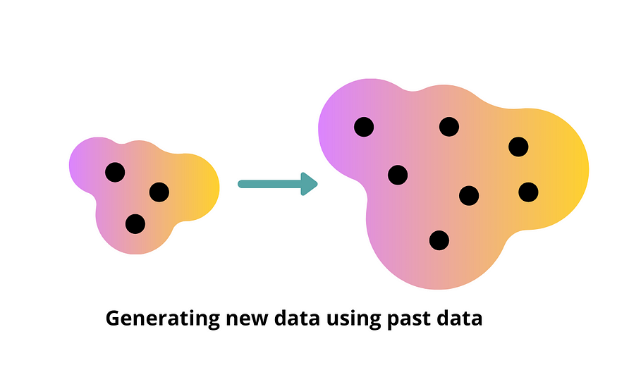
Generative models are a type of machine learning model that can create new data based on the patterns and structure of existing data. Generative models learn the underlying distribution of the data and can generate new samples that are similar to the original data. Generative models are useful in scenarios where the data is limited or where the generation of new data is required.

Generative Models in Python

Python is a popular language for machine learning, and several libraries support generative models. In this tutorial, we will use the Keras library to build and train a generative model in Python.

Import Libraries

We will start by importing the necessary libraries, including Keras for generative models, and NumPy and Matplotlib for data processing and visualization.

import numpy as np
import matplotlib.pyplot as plt
from keras.layers import Input, Dense, Reshape, Flatten
from keras.layers.advanced_activations import LeakyReLU
from keras.models import Sequential, Model
from keras.optimizers import Adam

Load Data

Next, we will load the data to train the generative model.

# Load data
(x_train, y_train), (_, _) = tf.keras.datasets.mnist.load_data()

# Normalize data
x_train = x_train / 255.0
# Flatten data
x_train = x_train.reshape(x_train.shape[0], -1)

In this example, we load the MNIST dataset and normalize and flatten the data.

Build Generative Model

Next, we will build the generative model.

# Build generative model
def build_generator():

# Define input layer
    input_layer = Input(shape=(100,))
    # Define hidden layers
    hidden_layer_1 = Dense(128)(input_layer)
    hidden_layer_1 = LeakyReLU(alpha=0.2)(hidden_layer_1)
    hidden_layer_2 = Dense(256)(hidden_layer_1)
    hidden_layer_2 = LeakyReLU(alpha=0.2)(hidden_layer_2)
    hidden_layer_3 = Dense(512)(hidden_layer_2)
    hidden_layer_3 = LeakyReLU(alpha=0.2)(hidden_layer_3)
    # Define output layer
    output_layer = Dense(784, activation='sigmoid')(hidden_layer_3)
    output_layer = Reshape((28, 28))(output_layer)
    # Define model
    model = Model(inputs=input_layer, outputs=output_layer)
    return model
generator = build_generator()
generator.summary()

In this example, we define a generator model with input layer, hidden layers, and output layer.

Train Generative Model

Next, we will train the generative model.

# Define loss function and optimizer
loss_function = 'binary_crossentropy'
optimizer = Adam(lr=0.0002, beta_1=0.5)

# Compile model
generator.compile(loss=loss_function, optimizer=optimizer)

# Train model
epochs = 10000
batch_size = 128

for epoch in range(epochs):

    # Select random real samples
    index = np.random.randint(0, x_train.shape[0], batch_size)
    real_samples = x_train[index]

    # Generate fake samples
    noise = np.random.normal(0, 1, (batch_size, 100))
    fake_samples = generator.predict(noise)

    # Train generator
    generator_loss = generator.train_on_batch(noise, real_samples)

    # Print progress
    print('Epoch: %d, Generator Loss: %f' % (epoch + 1, generator_loss))

In this example, we define the loss function and optimizer, compile the model, and train the generator model on real and fake samples.

Generate New Data

Finally, we can use the trained generator model to generate new data.

# Generate new data
noise = np.random.normal(0, 1, (10, 100))
generated_samples = generator.predict(noise)

# Plot generated samples
for i in range(generated_samples.shape[0]):
    plt.imshow(generated_samples[i], cmap='gray')
    plt.axis('off')
    plt.show()

In this example, we generate 10 new data samples using the trained generator model and plot the samples.

In this tutorial, we covered the basics of generative models and how to use them in Python to create new data based on the patterns and structure of existing data. Generative models are useful in scenarios where the data is limited or where the generation of new data is required.

I hope you found this tutorial useful in understanding generative models in Python.

Building Your First Kubeflow Pipeline: A Simple Example

Building Your First Kubeflow Pipeline: A Simple Example

Kubeflow Pipelines is a powerful platform for building, deploying, and managing end-to-end machine learning workflows. It simplifies the process of creating and executing ML pipelines, making it easier for data scientists and engineers to collaborate on model development and deployment. In this tutorial, we will guide you through building and running a simple Kubeflow Pipeline using Python.

Prerequisites

  1. Familiarity with Python programming

Step 1: Install Kubeflow Pipelines SDK

First, you need to install the Kubeflow Pipelines SDK on your local machine. Run the following command in your terminal or command prompt:

pip install kfp

Step 2: Create a Simple Pipeline in Python

Create a new Python script (e.g., my_first_pipeline.py) and add the following code:

import kfp
from kfp import dsl

def load_data_op():
    return dsl.ContainerOp(
        name="Load Data",
        image="python:3.7",
        command=["sh", "-c"],
        arguments=["echo 'Loading data' && sleep 5"],
    )
def preprocess_data_op():
    return dsl.ContainerOp(
        name="Preprocess Data",
        image="python:3.7",
        command=["sh", "-c"],
        arguments=["echo 'Preprocessing data' && sleep 5"],
    )
def train_model_op():
    return dsl.ContainerOp(
        name="Train Model",
        image="python:3.7",
        command=["sh", "-c"],
        arguments=["echo 'Training model' && sleep 5"],
    )
@dsl.pipeline(
    name="My First Pipeline",
    description="A simple pipeline that demonstrates loading, preprocessing, and training steps."
)
def my_first_pipeline():
    load_data = load_data_op()
    preprocess_data = preprocess_data_op().after(load_data)
    train_model = train_model_op().after(preprocess_data)
if __name__ == "__main__":
    kfp.compiler.Compiler().compile(my_first_pipeline, "my_first_pipeline.yaml")

This Python script defines a simple pipeline with three steps: loading data, preprocessing data, and training a model. Each step is defined as a function that returns a ContainerOp object, which represents a containerized operation in the pipeline. The @dsl.pipeline decorator is used to define the pipeline, and the kfp.compiler.Compiler().compile() function is used to compile the pipeline into a YAML file.

Step 3: Upload and Run the Pipeline

  1. Click on the “Pipelines” tab in the left-hand sidebar.
  2. Click the “Upload pipeline” button in the upper right corner.
  3. In the “Upload pipeline” dialog, click “Browse” and select the my_first_pipeline.yaml file generated in the previous step.
  4. Click “Upload” to upload the pipeline to the Kubeflow platform.
  5. Once the pipeline is uploaded, click on its name to open the pipeline details page.
  6. Click the “Create run” button to start a new run of the pipeline.
  7. On the “Create run” page, you can give your run a name and choose a pipeline version. Click “Start” to begin the pipeline run.

Step 4: Monitor the Pipeline Run

After starting the pipeline run, you will be redirected to the “Run details” page. Here, you can monitor the progress of your pipeline, view the logs for each step, and inspect the output artifacts.

  1. To view the logs for a specific step, click on the step in the pipeline graph and then click the “Logs” tab in the right-hand pane.
  2. To view the output artifacts, click on the step in the pipeline graph and then click the “Artifacts” tab in the right-hand pane.

Congratulations! You have successfully built and executed your first Kubeflow Pipeline using Python. You can now experiment with more complex pipelines, integrate different components, and optimize your machine learning workflows.

With Kubeflow Pipelines, you can automate your machine learning workflows, making it easier to build, deploy, and manage complex ML models. Now that you have a basic understanding of how to create and run pipelines in Kubeflow, you can explore more advanced features and build more sophisticated pipelines for your own projects.

Kubeflow Pipelines: A Step-by-Step Guide

Kubeflow Pipelines: A Step-by-Step Guide

Kubeflow Pipelines is a platform for building, deploying, and managing end-to-end machine learning workflows. It streamlines the process of creating and executing ML pipelines, making it easier for data scientists and engineers to collaborate on model development and deployment. In this tutorial, we will guide you through the process of setting up Kubeflow Pipelines on your local machine using MiniKF and running a simple pipeline in Python.

Prerequisites

Step 1: Install Vagrant

First, you need to install Vagrant on your machine. Follow the installation instructions for your operating system here: https://www.vagrantup.com/docs/installation

Step 2: Set up MiniKF

Now, let’s set up MiniKF (Mini Kubeflow) on your local machine. MiniKF is a lightweight version of Kubeflow that runs on top of VirtualBox using Vagrant. It is perfect for testing and development purposes.

Create a new directory for your MiniKF setup and navigate to it in your terminal:

mkdir minikf
cd minikf

Initialize the MiniKF Vagrant box by running:

vagrant init arrikto/minikf

Start the MiniKF virtual machine:

vagrant up

This process will take some time, as Vagrant downloads the MiniKF box and sets up the virtual machine.

Step 3: Access the Kubeflow Dashboard

After the virtual machine is up and running, you can access the Kubeflow dashboard in your browser. Open the following URL: http://10.10.10.10. You will be prompted to log in with a username and password. Use admin as both the username and password.

Step 4: Create a Simple Pipeline in Python

Now, let’s create a simple pipeline in Python that reads some data, processes it, and outputs the result. First, install the Kubeflow Pipelines SDK:

pip install kfp

Create a new Python script (e.g., simple_pipeline.py) and add the following code:

import kfp
from kfp import dsl

def read_data_op():
    return dsl.ContainerOp(
        name="Read Data",
        image="python:3.7",
        command=["sh", "-c"],
        arguments=["echo 'Reading data' && sleep 5"],
    )
def process_data_op():
    return dsl.ContainerOp(
        name="Process Data",
        image="python:3.7",
        command=["sh", "-c"],
        arguments=["echo 'Processing data' && sleep 5"],
    )
def output_data_op():
    return dsl.ContainerOp(
        name="Output Data",
        image="python:3.7",
        command=["sh", "-c"],
        arguments=["echo 'Outputting data' && sleep 5"],
    )
@dsl.pipeline(
    name="Simple Pipeline",
    description="A simple pipeline that reads, processes, and outputs data."
)
def simple_pipeline():
    read_data = read_data_op()
    process_data = process_data_op().after(read_data)
    output_data = output_data_op().after(process_data)
if __name__ == "__main__":
    kfp.compiler.Compiler().compile(simple_pipeline, "simple_pipeline.yaml")

This Python script defines a simple pipeline with three steps: reading data, processing data, and outputting data. Each step is defined as a function that returns a ContainerOp object, which represents a containerized operation in the pipeline. The @dsl.pipeline decorator is used to define the pipeline, and the kfp.compiler.Compiler().compile() function is used to compile the pipeline into a YAML file.

Step 5: Upload and Run the Pipeline

Now that you have created a simple pipeline in Python, let’s upload and run it on the Kubeflow Pipelines platform.

Step 6: Monitor the Pipeline Run

After starting the pipeline run, you will be redirected to the “Run details” page. Here, you can monitor the progress of your pipeline, view the logs for each step, and inspect the output artifacts.

Congratulations! You have successfully set up Kubeflow Pipelines on your local machine, created a simple pipeline in Python, and executed it using the Kubeflow platform. You can now experiment with more complex pipelines, integrate different components, and optimize your machine learning workflows.

With Kubeflow Pipelines, you can automate your machine learning workflows, making it easier to build, deploy, and manage complex ML models. Now that you have a basic understanding of how to create and run pipelines in Kubeflow, you can explore more advanced features and build more sophisticated pipelines for your own projects.