Posts Tagged

python

Optimizing Model Performance: A Guide to Hyperparameter Tuning in Python with Keras

April 14, 2023 Model optimization Python

Optimizing Model Performance: A Guide to Hyperparameter Tuning in Python with Keras

Hyperparameter tuning is the process of selecting the best set of hyperparameters for a machine learning model to optimize its performance. Hyperparameters are values that cannot be learned from the data, but are set by the user before training the model. Examples of hyperparameters include learning rate, batch size, number of hidden layers, and number of neurons in each hidden layer.

Optimizing hyperparameters is important because it can significantly improve the performance of a machine learning model. However, it can be a time-consuming and computationally expensive process.

In this tutorial, we will use Python to demonstrate how to perform hyperparameter tuning using the Keras library.

Hyperparameter Tuning in Python with Keras

Import Libraries

We will start by importing the necessary libraries, including Keras for building the model and scikit-learn for hyperparameter tuning.

import numpy as np
from keras.datasets import mnist
from keras.models import Sequential
from keras.layers import Dense, Dropout
from keras.utils import to_categorical
from keras.optimizers import Adam
from sklearn.model_selection import RandomizedSearchCV

Load Data

Next, we will load the MNIST dataset for training and testing the model.

# Load data
(x_train, y_train), (x_test, y_test) = mnist.load_data()

# Normalize data
x_train = x_train.astype('float32') / 255.
x_test = x_test.astype('float32') / 255.
# Flatten data
x_train = x_train.reshape((len(x_train), np.prod(x_train.shape[1:])))
x_test = x_test.reshape((len(x_test), np.prod(x_test.shape[1:])))
# One-hot encode labels
y_train = to_categorical(y_train)
y_test = to_categorical(y_test)

In this example, we load the MNIST dataset and normalize and flatten the data. We also one-hot encode the labels.

Build Model

Next, we will build the model.

# Define model
def build_model(learning_rate=0.01, dropout_rate=0.0, neurons=64):

model = Sequential()
    model.add(Dense(neurons, activation='relu', input_shape=(784,)))
    model.add(Dropout(dropout_rate))
    model.add(Dense(neurons, activation='relu'))
    model.add(Dropout(dropout_rate))
    model.add(Dense(10, activation='softmax'))
    optimizer = Adam(lr=learning_rate)
    model.compile(loss='categorical_crossentropy', optimizer=optimizer, metrics=['accuracy'])
    return model

In this example, we define the model with three layers, including two hidden layers with a user-defined number of neurons and a dropout layer for regularization.

Perform Hyperparameter Tuning

Next, we will perform hyperparameter tuning using scikit-learn’s RandomizedSearchCV function.

# Define hyperparameters
params = {
    'learning_rate': [0.01, 0.001, 0.0001],
    'dropout_rate': [0.0, 0.1, 0.2],
    'neurons': [32, 64, 128],
    'batch_size': [32, 64, 128]
}

# Create model
model = build_model()
# Perform hyperparameter tuning
random_search = RandomizedSearchCV(model, param_distributions=params, cv=3)
random_search.fit(x_train, y_train)
# Print best hyperparameters
print(random_search.best_params_)

In this example, we define a dictionary of hyperparameters and their values to be tuned. We then create the model and perform hyperparameter tuning using RandomizedSearchCV with a 3-fold cross-validation. Finally, we print the best hyperparameters found during the tuning process.

Evaluate Model

Once we have found the best hyperparameters, we can build the final model with those hyperparameters and evaluate its performance on the testing data.

# Build final model with best hyperparameters
best_learning_rate = random_search.best_params_['learning_rate']
best_dropout_rate = random_search.best_params_['dropout_rate']
best_neurons = random_search.best_params_['neurons']
model = build_model(learning_rate=best_learning_rate, dropout_rate=best_dropout_rate, neurons=best_neurons)

# Train model
model.fit(x_train, y_train, batch_size=128, epochs=10, validation_data=(x_test, y_test))
# Evaluate model on testing data
score = model.evaluate(x_test, y_test, verbose=0)
print('Test loss:', score[0])
print('Test accuracy:', score[1])

In this example, we build the final model with the best hyperparameters found during hyperparameter tuning. We then train the model and evaluate its performance on the testing data.

In this tutorial, we covered the basics of hyperparameter tuning and how to perform it using Python with Keras and scikit-learn. By tuning the hyperparameters, we can significantly improve the performance of a machine learning model. I hope you found this tutorial useful in understanding how to optimize model performance through hyperparameter tuning.

LyronFoster

Lyron Foster is a Hawai’i based African American Author, Musician, Actor, Blogger, Philanthropist and Multinational Serial Tech Entrepreneur.

lyronfoster.com

Creating New Data with Generative Models in Python

April 13, 2023 Keras Machine Learning Python

Creating New Data with Generative Models in Python

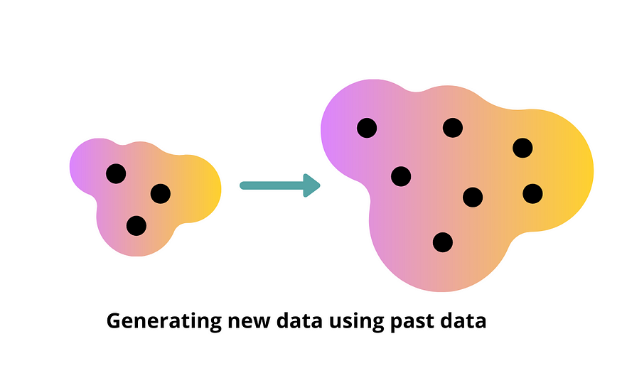
Generative models are a type of machine learning model that can create new data based on the patterns and structure of existing data. Generative models learn the underlying distribution of the data and can generate new samples that are similar to the original data. Generative models are useful in scenarios where the data is limited or where the generation of new data is required.

Generative Models in Python

Python is a popular language for machine learning, and several libraries support generative models. In this tutorial, we will use the Keras library to build and train a generative model in Python.

Import Libraries

We will start by importing the necessary libraries, including Keras for generative models, and NumPy and Matplotlib for data processing and visualization.

import numpy as np
import matplotlib.pyplot as plt
from keras.layers import Input, Dense, Reshape, Flatten
from keras.layers.advanced_activations import LeakyReLU
from keras.models import Sequential, Model
from keras.optimizers import Adam

Load Data

Next, we will load the data to train the generative model.

# Load data
(x_train, y_train), (_, _) = tf.keras.datasets.mnist.load_data()

# Normalize data
x_train = x_train / 255.0
# Flatten data
x_train = x_train.reshape(x_train.shape[0], -1)

In this example, we load the MNIST dataset and normalize and flatten the data.

Build Generative Model

Next, we will build the generative model.

# Build generative model
def build_generator():

# Define input layer
    input_layer = Input(shape=(100,))
    # Define hidden layers
    hidden_layer_1 = Dense(128)(input_layer)
    hidden_layer_1 = LeakyReLU(alpha=0.2)(hidden_layer_1)
    hidden_layer_2 = Dense(256)(hidden_layer_1)
    hidden_layer_2 = LeakyReLU(alpha=0.2)(hidden_layer_2)
    hidden_layer_3 = Dense(512)(hidden_layer_2)
    hidden_layer_3 = LeakyReLU(alpha=0.2)(hidden_layer_3)
    # Define output layer
    output_layer = Dense(784, activation='sigmoid')(hidden_layer_3)
    output_layer = Reshape((28, 28))(output_layer)
    # Define model
    model = Model(inputs=input_layer, outputs=output_layer)
    return model
generator = build_generator()
generator.summary()

In this example, we define a generator model with input layer, hidden layers, and output layer.

Train Generative Model

Next, we will train the generative model.

# Define loss function and optimizer
loss_function = 'binary_crossentropy'
optimizer = Adam(lr=0.0002, beta_1=0.5)

# Compile model
generator.compile(loss=loss_function, optimizer=optimizer)

# Train model
epochs = 10000
batch_size = 128

for epoch in range(epochs):

    # Select random real samples
    index = np.random.randint(0, x_train.shape[0], batch_size)
    real_samples = x_train[index]

    # Generate fake samples
    noise = np.random.normal(0, 1, (batch_size, 100))
    fake_samples = generator.predict(noise)

    # Train generator
    generator_loss = generator.train_on_batch(noise, real_samples)

    # Print progress
    print('Epoch: %d, Generator Loss: %f' % (epoch + 1, generator_loss))

In this example, we define the loss function and optimizer, compile the model, and train the generator model on real and fake samples.

Generate New Data

Finally, we can use the trained generator model to generate new data.

# Generate new data
noise = np.random.normal(0, 1, (10, 100))
generated_samples = generator.predict(noise)

# Plot generated samples
for i in range(generated_samples.shape[0]):
    plt.imshow(generated_samples[i], cmap='gray')
    plt.axis('off')
    plt.show()

In this example, we generate 10 new data samples using the trained generator model and plot the samples.

In this tutorial, we covered the basics of generative models and how to use them in Python to create new data based on the patterns and structure of existing data. Generative models are useful in scenarios where the data is limited or where the generation of new data is required.

I hope you found this tutorial useful in understanding generative models in Python.

LyronFoster

Lyron Foster is a Hawai’i based African American Author, Musician, Actor, Blogger, Philanthropist and Multinational Serial Tech Entrepreneur.

lyronfoster.com

Kubeflow Pipelines: A Step-by-Step Guide

April 11, 2023 artificial intelligence Kubeflow kubernetes Machine Learning Python

Kubeflow Pipelines: A Step-by-Step Guide

Kubeflow Pipelines is a platform for building, deploying, and managing end-to-end machine learning workflows. It streamlines the process of creating and executing ML pipelines, making it easier for data scientists and engineers to collaborate on model development and deployment. In this tutorial, we will guide you through the process of setting up Kubeflow Pipelines on your local machine using MiniKF and running a simple pipeline in Python.

Prerequisites

A computer with at least 8GB RAM and 50GB of free disk space
VirtualBox installed (Download from https://www.virtualbox.org/wiki/Downloads)
MiniKF Vagrant box downloaded (Download from https://www.vagrantup.com/docs/boxes)

Step 1: Install Vagrant

First, you need to install Vagrant on your machine. Follow the installation instructions for your operating system here: https://www.vagrantup.com/docs/installation

Step 2: Set up MiniKF

Now, let’s set up MiniKF (Mini Kubeflow) on your local machine. MiniKF is a lightweight version of Kubeflow that runs on top of VirtualBox using Vagrant. It is perfect for testing and development purposes.

Create a new directory for your MiniKF setup and navigate to it in your terminal:

mkdir minikf
cd minikf

Initialize the MiniKF Vagrant box by running:

vagrant init arrikto/minikf

Start the MiniKF virtual machine:

vagrant up

This process will take some time, as Vagrant downloads the MiniKF box and sets up the virtual machine.

Step 3: Access the Kubeflow Dashboard

After the virtual machine is up and running, you can access the Kubeflow dashboard in your browser. Open the following URL: http://10.10.10.10. You will be prompted to log in with a username and password. Use admin as both the username and password.

Step 4: Create a Simple Pipeline in Python

Now, let’s create a simple pipeline in Python that reads some data, processes it, and outputs the result. First, install the Kubeflow Pipelines SDK:

pip install kfp

Create a new Python script (e.g., simple_pipeline.py) and add the following code:

import kfp
from kfp import dsl

def read_data_op():
    return dsl.ContainerOp(
        name="Read Data",
        image="python:3.7",
        command=["sh", "-c"],
        arguments=["echo 'Reading data' && sleep 5"],
    )
def process_data_op():
    return dsl.ContainerOp(
        name="Process Data",
        image="python:3.7",
        command=["sh", "-c"],
        arguments=["echo 'Processing data' && sleep 5"],
    )
def output_data_op():
    return dsl.ContainerOp(
        name="Output Data",
        image="python:3.7",
        command=["sh", "-c"],
        arguments=["echo 'Outputting data' && sleep 5"],
    )
@dsl.pipeline(
    name="Simple Pipeline",
    description="A simple pipeline that reads, processes, and outputs data."
)
def simple_pipeline():
    read_data = read_data_op()
    process_data = process_data_op().after(read_data)
    output_data = output_data_op().after(process_data)
if __name__ == "__main__":
    kfp.compiler.Compiler().compile(simple_pipeline, "simple_pipeline.yaml")

This Python script defines a simple pipeline with three steps: reading data, processing data, and outputting data. Each step is defined as a function that returns a ContainerOp object, which represents a containerized operation in the pipeline. The @dsl.pipeline decorator is used to define the pipeline, and the kfp.compiler.Compiler().compile() function is used to compile the pipeline into a YAML file.

Step 5: Upload and Run the Pipeline

Now that you have created a simple pipeline in Python, let’s upload and run it on the Kubeflow Pipelines platform.

Go to the Kubeflow dashboard (http://10.10.10.10) and click on the “Pipelines” tab in the left-hand sidebar.
Click the “Upload pipeline” button in the upper right corner.
In the “Upload pipeline” dialog, click “Browse” and select the simple_pipeline.yaml file generated in the previous step.
Click “Upload” to upload the pipeline to the Kubeflow platform.
Once the pipeline is uploaded, click on its name to open the pipeline details page.
Click the “Create run” button to start a new run of the pipeline.
On the “Create run” page, you can give your run a name and choose a pipeline version. Click “Start” to begin the pipeline run.

Step 6: Monitor the Pipeline Run

After starting the pipeline run, you will be redirected to the “Run details” page. Here, you can monitor the progress of your pipeline, view the logs for each step, and inspect the output artifacts.

The pipeline graph will show the status of each step in the pipeline, with different colors indicating success, failure, or in-progress status.
To view the logs for a specific step, click on the step in the pipeline graph and then click the “Logs” tab in the right-hand pane.
To view the output artifacts, click on the step in the pipeline graph and then click the “Artifacts” tab in the right-hand pane.

Congratulations! You have successfully set up Kubeflow Pipelines on your local machine, created a simple pipeline in Python, and executed it using the Kubeflow platform. You can now experiment with more complex pipelines, integrate different components, and optimize your machine learning workflows.

With Kubeflow Pipelines, you can automate your machine learning workflows, making it easier to build, deploy, and manage complex ML models. Now that you have a basic understanding of how to create and run pipelines in Kubeflow, you can explore more advanced features and build more sophisticated pipelines for your own projects.

LyronFoster

Lyron Foster is a Hawai’i based African American Author, Musician, Actor, Blogger, Philanthropist and Multinational Serial Tech Entrepreneur.

lyronfoster.com

AutoML: Automated Machine Learning in Python

April 11, 2023 artificial intelligence Machine Learning Python Technical Stuff

AutoML: Automated Machine Learning in Python

AutoML (Automated Machine Learning) is a branch of machine learning that uses artificial intelligence and machine learning techniques to automate the entire machine learning process. AutoML automates tasks such as data preparation, feature engineering, algorithm selection, hyperparameter tuning, and model evaluation. AutoML enables non-experts to build and deploy machine learning models with minimal effort and technical knowledge.

Automated Machine Learning in Python

Python is a popular language for machine learning, and several libraries support AutoML. In this tutorial, we will use the H2O library to perform AutoML in Python.

Install Library

We will start by installing the H2O library.

pip install h2o

Import Libraries

Next, we will import the necessary libraries, including H2O for AutoML, and NumPy and Pandas for data processing.

import numpy as np
import pandas as pd
import h2o
from h2o.automl import H2OAutoML

Load Data

Next, we will load the data to train the AutoML model

# Load data
url = "https://archive.ics.uci.edu/ml/machine-learning-databases/iris/iris.data"
data = pd.read_csv(url, header=None, names=['sepal_length', 'sepal_width', 'petal_length', 'petal_width', 'class'])

# Convert data to H2O format
h2o.init()
h2o_data = h2o.H2OFrame(data)

In this example, we load the Iris dataset from a URL and convert it to the H2O format.

Train AutoML Model

Next, we will train an AutoML model on the data.

# Train AutoML model
aml = H2OAutoML(max_models=10, seed=1)
aml.train(x=['sepal_length', 'sepal_width', 'petal_length', 'petal_width'], y='class', training_frame=h2o_data)

In this example, we train an AutoML model with a maximum of 10 models and a random seed of 1.

View Model Leaderboard

Next, we can view the leaderboard of the trained models.

# View model leaderboard
lb = aml.leaderboard
print(lb)

In this example, we print the leaderboard of the trained models.

Test AutoML Model

Finally, we can use the trained AutoML model to make predictions on new data.

# Test AutoML model
test_data = pd.DataFrame(np.array([[5.1, 3.5, 1.4, 0.2], [7.7, 3.0, 6.1, 2.3]]), columns=['sepal_length', 'sepal_width', 'petal_length', 'petal_width'])
h2o_test_data = h2o.H2OFrame(test_data)
preds = aml.predict(h2o_test_data)
print(preds)

In this example, we use the trained AutoML model to predict the class of two new data points.

In this tutorial, we covered the basics of AutoML and how to use it in Python to automate the entire machine learning process. AutoML enables non-experts to build and deploy machine learning models with minimal effort and technical knowledge. I hope you found this tutorial useful in understanding AutoML in Python.

LyronFoster

Lyron Foster is a Hawai’i based African American Author, Musician, Actor, Blogger, Philanthropist and Multinational Serial Tech Entrepreneur.

lyronfoster.com

Defending Your Web Application: Understanding and Preventing SQL Injection Attacks

April 11, 2023 Cyber Security Python Technical Stuff

Defending Your Web Application: Understanding and Preventing SQL Injection Attacks

SQL injection attacks are one of the most common types of web application attacks that can compromise the security of your website or application. These attacks can be used to gain unauthorized access to sensitive data, modify data, or execute malicious code. In this tutorial, we will explain what SQL injection attacks are, how they work, and how you can prevent them.

What is SQL Injection?

SQL injection is a type of attack where an attacker exploits a vulnerability in a web application’s input validation and uses it to inject malicious SQL code into the application’s database. This malicious SQL code can be used to manipulate or extract data from the database, or even execute arbitrary code on the server.

How does SQL Injection work?

SQL injection attacks work by taking advantage of input validation vulnerabilities in web applications. In most web applications, user input is used to build SQL queries that are executed on the server-side. If this input is not properly validated, an attacker can manipulate the input to include their own SQL code.

For example, consider a login form that asks the user for their username and password. If the application uses the following SQL query to validate the user’s credentials:

SELECT * FROM users WHERE username='username' AND password='password'

An attacker could use a SQL injection attack by entering the following as the password:

' OR 1=1 --

This would result in the following SQL query being executed on the server:

SELECT * FROM users WHERE username='username' AND password='' OR 1=1 --'

The -- at the end of the password input is used to comment out the rest of the query, so the attacker can avoid syntax errors. In this case, the attacker has successfully bypassed the login form and gained access to the application.

Preventing SQL Injection Attacks

There are several ways to prevent SQL injection attacks. Here are some best practices:

Use Parameterized Queries: Parameterized queries are a type of prepared statement that allows you to separate the SQL code from the user input. This means that the input is treated as a parameter, and not as part of the SQL query. This approach can help prevent SQL injection attacks by ensuring that the user input is not executed as SQL code. Here’s an example of a parameterized query in Python using the sqlite3 module:

import sqlite3

conn = sqlite3.connect('example.db')
c = conn.cursor()
username = 'username'
password = 'password'
c.execute('SELECT * FROM users WHERE username=? AND password=?', (username, password))

Validate User Input: User input should always be validated to ensure that it matches the expected format and does not contain malicious code. Regular expressions can be used to validate input for specific formats (e.g. email addresses or phone numbers). You should also sanitize user input by removing any special characters that could be used to inject malicious SQL code.

Use Stored Procedures: Stored procedures are precompiled SQL statements that can be called from within the application. This approach can help prevent SQL injection attacks by ensuring that the user input is not executed as SQL code. However, it’s important to ensure that the stored procedures themselves are secure and cannot be manipulated by an attacker.

Use an ORM: Object-relational mapping (ORM) frameworks like SQLAlchemy can help prevent SQL injection attacks by abstracting the SQL code away from the application code. The ORM handles the construction and execution of SQL queries based on the application’s object model, which can help prevent SQL injection attacks.

SQL injection attacks can have serious consequences for web applications and their users. By following the best practices outlined in this tutorial, you can help prevent SQL injection attacks and ensure the security of your application’s database. Remember to always validate user input, use parameterized queries, and consider using an ORM or stored procedures to help prevent SQL injection attacks.

Python Code Example

Here’s a Python code example that demonstrates a simple SQL injection attack and how to prevent it using parameterized queries:

import sqlite3

conn = sqlite3.connect('example.db')
c = conn.cursor()
# Login form
username = input('Username: ')
password = input('Password: ')
# Vulnerable query
query = "SELECT * FROM users WHERE username = '%s' AND password = '%s'" % (username, password)
# Malicious password input
password = "' OR 1=1 --"
# Malicious query
malicious_query = "SELECT * FROM users WHERE username = '%s' AND password = '%s'" % (username, password)
# Vulnerable query execution
print("Executing vulnerable query:")
c.execute(query)
print(c.fetchone())
# Malicious query execution
print("\nExecuting malicious query:")
c.execute(malicious_query)
print(c.fetchone())
# Preventing SQL injection with parameterized queries
print("\nPreventing SQL injection with parameterized queries:")
c.execute("SELECT * FROM users WHERE username = ? AND password = ?", (username, password))
print(c.fetchone())

In this example, we first prompt the user for their username and password. We then create a vulnerable SQL query that concatenates the user input into the SQL string. We also create a malicious input that will allow the attacker to bypass the login form. We execute both the vulnerable and malicious queries and print the results.

Finally, we prevent SQL injection by using a parameterized query. We pass the user input as parameters to the query using a tuple, which allows the input to be properly sanitized and prevents the attacker from injecting malicious SQL code.

By following best practices like parameterized queries and input validation, you can prevent SQL injection attacks and protect your web application’s database.

LyronFoster

Lyron Foster is a Hawai’i based African American Author, Musician, Actor, Blogger, Philanthropist and Multinational Serial Tech Entrepreneur.

lyronfoster.com

Bayesian Machine Learning: Probabilistic Models and Inference in Python

April 11, 2023 Machine Learning Python Technical Stuff

Bayesian Machine Learning: Probabilistic Models and Inference in Python

Bayesian Machine Learning is a branch of machine learning that incorporates probability theory and Bayesian inference in its models. Bayesian Machine Learning enables the estimation of model parameters and prediction uncertainty through probabilistic models and inference techniques. Bayesian Machine Learning is useful in scenarios where uncertainty is high and where the data is limited or noisy.

Probabilistic Models and Inference in Python

Python is a popular language for machine learning, and several libraries support Bayesian Machine Learning. In this tutorial, we will use the PyMC3 library to build and fit probabilistic models and perform Bayesian inference.

Import Libraries

We will start by importing the necessary libraries, including NumPy for numerical computations, Matplotlib for visualizations, and PyMC3 for probabilistic models and inference.

import numpy as np
import matplotlib.pyplot as plt
import pymc3 as pm

Generate Data

Next, we will generate some random data to fit our probabilistic model.

# Generate random data
np.random.seed(1)
x = np.linspace(0, 10, 50)
y = 2*x + 1 + np.random.randn(50)

In this example, we generate 50 data points with a linear relationship between x and y.

Build Probabilistic Model

Next, we will build a probabilistic model to fit the data.

# Build probabilistic model
with pm.Model() as model:
    # Define priors
    alpha = pm.Normal('alpha', mu=0, sd=10)
    beta = pm.Normal('beta', mu=0, sd=10)
    sigma = pm.HalfNormal('sigma', sd=1)

# Define likelihood
    y_obs = pm.Normal('y_obs', mu=alpha + beta*x, sd=sigma, observed=y)

In this example, we define the priors for the model parameters (alpha, beta, and sigma) and the likelihood for the data.

Fit Probabilistic Model

Next, we will fit the probabilistic model to the data using Bayesian inference.

# Fit probabilistic model
with model:
    # Sample from posterior distribution
    trace = pm.sample(1000)

# Plot posterior distributions
pm.plot_posterior(trace, var_names=['alpha', 'beta', 'sigma'])
plt.show()

In this example, we use the sample function from PyMC3 to sample from the posterior distribution of the model parameters. We then plot the posterior distributions of the parameters.

Make Predictions

Finally, we can use the fitted probabilistic model to make predictions on new data.

# Make predictions
x_new = np.linspace(0, 10, 100)
with model:
    # Predict y values for new x values
    y_new = pm.sample_posterior_predictive(trace, var_names=['y_obs'], samples=100, \
        model=model, inputs={'x': x_new})

# Plot predictions
plt.scatter(x, y)
plt.plot(x_new, np.mean(y_new['y_obs'], axis=0), color='red')
plt.fill_between(x_new, np.percentile(y_new['y_obs'], 2.5, axis=0), \
    np.percentile(y_new['y_obs'], 97.5, axis=0), color='red', alpha=0.2)
plt.show()

In this example, we use the sample_posterior_predictive function from PyMC3 to predict y values for new x values. We then plot the predictions and the associated uncertainty.

In this tutorial, we covered the basics of Bayesian Machine Learning and how to use it in Python to build and fit probabilistic models and perform Bayesian inference. Bayesian Machine Learning enables the estimation of model parameters and prediction uncertainty through probabilistic models and inference techniques. It is useful in scenarios where uncertainty is high and where the data is limited or noisy. I hope you found this tutorial useful in understanding Bayesian Machine Learning in Python.

Note

The code examples provided in this tutorial are for illustrative purposes only and are not intended for production use. The code should be adapted to specific use cases and may require additional validation and testing.

LyronFoster

Lyron Foster is a Hawai’i based African American Author, Musician, Actor, Blogger, Philanthropist and Multinational Serial Tech Entrepreneur.

lyronfoster.com

Multi-Threading and Concurrency in Python

April 11, 2023 Multi-threading Python

Multi-Threading and Concurrency in Python

Python is a popular programming language that is known for its simplicity, readability, and flexibility. One of its strengths is its support for concurrency and multi-threading, which allows developers to write programs that can perform multiple tasks at the same time.

In this tutorial, we will explore multi-threading and concurrency in Python, including how to create and manage threads, synchronize data between threads, and handle common issues that arise when working with multiple threads.

Understanding Multi-threading and Concurrency

Concurrency is the ability of a program to perform multiple tasks at the same time, while multi-threading is a specific implementation of concurrency that allows a program to run multiple threads of execution within a single process. In Python, each thread runs independently and can perform different tasks concurrently. However, since threads share the same memory space, they can also access and modify the same data at the same time, which can lead to race conditions, deadlocks, and other synchronization issues.

Creating Threads in Python

Python provides built-in support for creating and managing threads using the threading module. To create a new thread, we can simply create an instance of the Thread class and pass in a function that the thread should run. Here’s an example:

import threading

def print_numbers():
    for i in range(10):
        print(i)
t = threading.Thread(target=print_numbers)
t.start()pyth

In this example, we create a new thread that runs the print_numbers function. We then start the thread using the start method, which begins executing the function in a separate thread. The output of this program will be a sequence of numbers from 0 to 9, printed by the main thread and the new thread concurrently.

Managing Threads in Python

Once we have created a thread, we can manage it using various methods provided by the threading module. For example, we can use the join method to wait for a thread to complete before continuing with the main thread:

import threading

def print_numbers():
    for i in range(10):
        print(i)
t = threading.Thread(target=print_numbers)
t.start()
t.join()
print("Done")

In this example, the main thread creates a new thread to run the print_numbers function. The join method is then called on the thread to wait for it to complete before printing “Done”.

Synchronizing Data between Threads in Python

One of the challenges of multi-threaded programming is managing shared data between threads. To avoid race conditions and other synchronization issues, we can use various synchronization primitives provided by the threading module, such as locks, semaphores, and events.

Here’s an example of using a lock to protect a shared variable between two threads:

import threading

counter = 0
lock = threading.Lock()
def increment():
    global counter
    for i in range(100000):
        with lock:
            counter += 1
t1 = threading.Thread(target=increment)
t2 = threading.Thread(target=increment)
t1.start()
t2.start()
t1.join()
t2.join()
print(counter)

In this example, we create a global counter variable that is shared between two threads. We also create a lock object using the Lock class, which can be used to synchronize access to the counter variable. The increment function is then defined to loop 100000 times and increment the counter variable by 1. However, the critical section that modifies the counter variable is protected by a with statement that acquires the lock before executing the critical section and releases the lock afterwards.

Handling Common Issues in Multi-threading

When working with multiple threads, there are several common issues that can arise, such as race conditions, deadlocks, and starvation. Here are some tips for handling these issues in Python:

Avoid shared state as much as possible: Shared state between threads can be a source of many problems. Whenever possible, try to use immutable data structures or thread-safe collections like queue.Queue to pass data between threads.

Use locks sparingly: While locks can be used to synchronize access to shared data, they can also introduce problems like deadlocks and performance issues. Use locks only when necessary and try to keep their critical sections as short as possible.

Use thread-local data where appropriate: Thread-local data is data that is local to a specific thread and is not shared between threads. This can be useful for storing thread-specific data like configuration settings or caches.

Use timeouts and non-blocking operations: When waiting for shared resources, use timeouts or non-blocking operations to avoid blocking other threads. This can help prevent deadlocks and improve performance.

Be aware of the Global Interpreter Lock (GIL): In Python, the GIL is a mechanism that ensures that only one thread can execute Python bytecode at a time. This means that multi-threading in Python does not provide true parallelism, and that CPU-bound tasks may not benefit from using multiple threads.

Multi-threading and concurrency are powerful features of Python that can help developers write more efficient and responsive programs. However, working with multiple threads also introduces new challenges and requires careful management of shared data and synchronization. By following best practices and being aware of common issues, developers can use multi-threading and concurrency to create faster, more responsive applications.

I hope this tutorial has been helpful in introducing you to multi-threading and concurrency in Python!

LyronFoster

Lyron Foster is a Hawai’i based African American Author, Musician, Actor, Blogger, Philanthropist and Multinational Serial Tech Entrepreneur.

lyronfoster.com

Active Learning: Learning with Limited Labeled Data in Python (Scikit-learn, Active Learning Lib)

April 9, 2023 artificial intelligence Machine Learning Technical Stuff

Active Learning: Learning with Limited Labeled Data in Python (Scikit-learn, Active Learning Lib)

Active Learning is a machine learning approach that enables the selection of the most informative data points to be labeled by an oracle, thereby reducing the number of labeled data points required to train a model. Active Learning is useful in scenarios where labeled data is limited or expensive to acquire. Active Learning can help improve the accuracy of machine learning models with fewer labeled data points.

Learning with Limited Labeled Data in Python

Python is a popular language for machine learning, and several libraries support Active Learning. In this tutorial, we will use the Scikit-learn library to train a model and the Active Learning library to select informative data points to be labeled.

Import Libraries

We will start by importing the necessary libraries, including Scikit-learn for training the model, NumPy for numerical computations, and the Active Learning library for selecting informative data points to be labeled.

import numpy as np
from sklearn.datasets import make_classification
from sklearn.linear_model import LogisticRegression
from sklearn.model_selection import train_test_split
from modAL.uncertainty import uncertainty_sampling

Generate Data

Next, we will generate some random data for training and testing the model.

# Generate random data for training and testing
X, y = make_classification(n_samples=1000, n_features=10, n_informative=5, n_classes=2, random_state=1)

In this example, we generate 1000 data points with 10 features and 5 informative features for training and testing.

Split Data

Next, we will split the data into a training set and a test set.

# Split data into training set and test set
X_train, X_test, y_train, y_test = train_test_split(X, y, test_size=0.2, random_state=1)

In this example, we split the data into a training set and a test set, with 20% of the data in the test set.

Train Initial Model

Next, we will train an initial logistic regression model on the labeled data.

# Train initial model
model = LogisticRegression()
model.fit(X_train[:10], y_train[:10])

In this example, we train an initial model on the first 10 labeled data points.

Active Learning

Next, we will use Active Learning to select informative data points to be labeled by an oracle.

# Active Learning
for i in range(10):
    # Select most informative data point to be labeled
    query_idx, query_inst = uncertainty_sampling(model, X_train)
    
    # Label data point
    y_new = np.array([int(input(f"Enter label for instance {j+1}: ")) for j in query_idx])
    
    # Add labeled data point to training data
    X_train = np.concatenate((X_train, query_inst.reshape(1, -1)))
    y_train = np.concatenate((y_train, y_new))
    
    # Retrain model
    model.fit(X_train, y_train)

In this example, we use the uncertainty_sampling function from the Active Learning library to select the most informative data point to be labeled by an oracle. We then ask the user to label the data point and add the labeled data point to the training data. We then retrain the model on the new labeled data.

Test Model

Finally, we will test the model on the test data.

# Test model
score = model.score(X_test, y_test)
print(f"Model accuracy: {score}")

In this example, we test the model on the test data and print the accuracy.

In this tutorial, we covered the basics of Active Learning and how to use it in Python to train machine learning models with limited labeled data. Active Learning is a useful approach in scenarios where labeled data is limited or expensive to acquire, and can help improve the accuracy of machine learning models with fewer labeled data points. I hope you found this tutorial useful in understanding Active Learning in Python.

LyronFoster

Lyron Foster is a Hawai’i based African American Author, Musician, Actor, Blogger, Philanthropist and Multinational Serial Tech Entrepreneur.

lyronfoster.com

Explainable AI: Interpreting Machine Learning Models in Python using LIME

April 8, 2023 artificial intelligence Machine Learning Python

Explainable AI: Interpreting Machine Learning Models in Python using LIME

Explainable AI (XAI) is an approach to machine learning that enables the interpretation and explanation of how a model makes decisions. This is important in cases where the model’s decision-making process needs to be transparent or explainable to humans, such as in medical diagnosis, financial forecasting, and legal decision-making. XAI techniques can help increase trust in machine learning models and improve their usability.

Interpreting Machine Learning Models in Python

Python is a popular language for machine learning, and several libraries support interpreting machine learning models. In this tutorial, we will use the Scikit-learn library to train a model and the LIME library to interpret the model’s predictions.

Import Libraries

We will start by importing the necessary libraries, including Scikit-learn for training the model, NumPy for numerical computations, and LIME for interpreting the model’s predictions.

import numpy as np
from sklearn.ensemble import RandomForestClassifier
from lime.lime_tabular import LimeTabularExplainer

Generate Data

Next, we will generate some random data for training and testing the model.

# Generate random data for training and testing
X_train = np.random.rand(100, 5)
y_train = np.random.randint(0, 2, size=(100,))
X_test = np.random.rand(50, 5)
y_test = np.random.randint(0, 2, size=(50,))

In this example, we generate 100 data points with 5 features for training and 50 data points with 5 features for testing. We also generate random binary labels for the data.

Train Model

Next, we will train a Random Forest model on the training data.

# Train model
model = RandomForestClassifier()
model.fit(X_train, y_train)

Interpret Model Predictions

Next, we will use LIME to interpret the model’s predictions on a test data point.

# Interpret model predictions
explainer = LimeTabularExplainer(X_train, feature_names=['feature'+str(i) for i in range(X_train.shape[1])], class_names=['0', '1'])
exp = explainer.explain_instance(X_test[0], model.predict_proba)

In this example, we use LimeTabularExplainer to create an explainer object and explain_instance to interpret the model’s predictions on the first test data point.

Visualize Interpretation

Finally, we will visualize the interpretation of the model’s predictions using a bar chart.

# Visualize interpretation
exp.show_in_notebook(show_table=True, show_all=False)

In this example, we use show_in_notebook to visualize the interpretation of the model’s predictions.

In this tutorial, we covered the basics of Explainable AI and how to interpret machine learning models using LIME in Python. XAI is an important area of research in machine learning, and XAI techniques can help improve the trust and transparency of machine learning models. I hope you found this tutorial useful in understanding Explainable AI in Python.

LyronFoster

Lyron Foster is a Hawai’i based African American Author, Musician, Actor, Blogger, Philanthropist and Multinational Serial Tech Entrepreneur.

lyronfoster.com

Unsupervised Learning: Clustering and Dimensionality Reduction in Python

April 8, 2023 artificial intelligence Machine Learning Python Technical Stuff

Unsupervised Learning: Clustering and Dimensionality Reduction in Python

Unsupervised learning is a type of machine learning where the model is not provided with labeled data. The model learns the underlying structure and patterns in the data without any specific guidance on what to look for. Clustering and Dimensionality Reduction are two important techniques in unsupervised learning.

Clustering

Clustering is a technique where the model tries to identify groups in the data based on their similarities. The objective is to group similar data points together and separate dissimilar data points. Clustering algorithms can be used for a variety of applications such as customer segmentation, anomaly detection, and image segmentation.

Dimensionality Reduction

Dimensionality reduction is a technique where the model tries to reduce the number of features in the data while retaining as much information as possible. This is useful when dealing with high-dimensional data where it’s difficult to visualize and analyze the data. Dimensionality reduction algorithms can be used for a variety of applications such as data compression, feature extraction, and visualization.

Clustering Algorithms

There are several clustering algorithms in machine learning, each with its own strengths and weaknesses. In this tutorial, we will cover two popular clustering algorithms: K-Means Clustering and Hierarchical Clustering.

K-Means Clustering

K-Means Clustering is a simple and efficient clustering algorithm. The algorithm partitions the data into K clusters based on their similarity. The number of clusters K is specified by the user. The algorithm starts by randomly selecting K data points as the initial centroids. The data points are then assigned to the nearest centroid based on their distance. The centroid is then updated based on the mean of the data points in the cluster. This process is repeated until convergence.

Let’s see how to implement K-Means Clustering in Python using Scikit-Learn.

from sklearn.cluster import KMeans
import numpy as np

# Generate random data
X = np.random.rand(100, 2)
# Initialize KMeans model with 2 clusters
kmeans = KMeans(n_clusters=2)
# Fit the model to the data
kmeans.fit(X)
# Predict the clusters for the data
y_pred = kmeans.predict(X)
# Print the centroids of the clusters
print(kmeans.cluster_centers_)

In this example, we generate random data with 2 features and 100 data points. We then initialize the KMeans model with 2 clusters and fit the model to the data. We then predict the clusters for the data and print the centroids of the clusters.

Hierarchical Clustering

Hierarchical Clustering is a clustering algorithm that builds a hierarchy of clusters. The algorithm starts by treating each data point as a separate cluster. The algorithm then iteratively merges the closest clusters based on their distance until all the data points belong to a single cluster.

There are two types of hierarchical clustering algorithms: Agglomerative and Divisive. Agglomerative clustering starts with each data point as a separate cluster and iteratively merges the closest clusters. Divisive clustering starts with all data points in a single cluster and iteratively splits the cluster into smaller clusters.

Let’s see how to implement Agglomerative Hierarchical Clustering in Python using Scikit-Learn.

from sklearn.cluster import AgglomerativeClustering
import numpy as np

# Generate random data
X = np.random.rand(100, 2)
# Initialize AgglomerativeClustering model with 2 clusters
agg_clustering = AgglomerativeClustering(n_clusters=2)
# Fit the model to the data
agg_clustering.fit(X)
# Predict the clusters for the data
y_pred = agg_clustering.labels_
# Print the labels of the clusters
print(y_pred)

In this example, we generate random data with 2 features and 100 data points. We then initialize the AgglomerativeClustering model with 2 clusters and fit the model to the data. We then predict the clusters for the data and print the labels of the clusters.

Divisive Hierarchical Clustering

Divisive Hierarchical Clustering is a clustering algorithm that starts with all data points in a single cluster and iteratively splits the cluster into smaller clusters. The algorithm starts by treating all data points as a single cluster. The algorithm then iteratively splits the cluster into smaller clusters based on their dissimilarity until each data point belongs to a separate cluster.

Divisive Hierarchical Clustering is not as popular as Agglomerative Hierarchical Clustering because it is computationally expensive and tends to produce imbalanced clusters.

Dimensionality Reduction Algorithms

There are several dimensionality reduction algorithms in machine learning, each with its own strengths and weaknesses. In this tutorial, we will cover two popular dimensionality reduction algorithms: Principal Component Analysis (PCA) and t-Distributed Stochastic Neighbor Embedding (t-SNE).

Principal Component Analysis (PCA)

Principal Component Analysis (PCA) is a linear dimensionality reduction technique that tries to find the orthogonal directions of maximum variance in the data. The objective is to find a lower-dimensional representation of the data that retains as much information as possible. PCA is useful when dealing with high-dimensional data where it’s difficult to visualize and analyze the data.

Let’s see how to implement PCA in Python using Scikit-Learn.

from sklearn.decomposition import PCA
import numpy as np

# Generate random data
X = np.random.rand(100, 10)
# Initialize PCA model with 2 components
pca = PCA(n_components=2)
# Fit the model to the data
pca.fit(X)
# Transform the data to 2 dimensions
X_transformed = pca.transform(X)
# Print the shape of the transformed data
print(X_transformed.shape)

In this example, we generate random data with 10 features and 100 data points. We then initialize the PCA model with 2 components and fit the model to the data. We then transform the data to 2 dimensions and print the shape of the transformed data.

t-Distributed Stochastic Neighbor Embedding (t-SNE)

t-Distributed Stochastic Neighbor Embedding (t-SNE) is a nonlinear dimensionality reduction technique that tries to preserve the pairwise distances between the data points in the lower-dimensional representation. The objective is to find a lower-dimensional representation of the data that retains the local structure of the data. t-SNE is useful when dealing with high-dimensional data where it’s difficult to visualize and analyze the data.

Let’s see how to implement t-SNE in Python using Scikit-Learn.

from sklearn.manifold import TSNE
import numpy as np

# Generate random data
X = np.random.rand(100, 10)
# Initialize t-SNE model with 2 components
tsne = TSNE(n_components=2)
# Fit the model to the data
X_transformed = tsne.fit_transform(X)
# Print the shape of the transformed data
print(X_transformed.shape)

In this example, we generate random data with 10 features and 100 data points. We then initialize the t-SNE model with 2 components and fit the model to the data. We then transform the data to 2 dimensions and print the shape of the transformed data.

In this tutorial, we covered two important techniques in unsupervised learning: Clustering and Dimensionality Reduction. We also covered two popular algorithms for each technique: K-Means Clustering and Hierarchical Clustering for Clustering, and PCA and t-SNE for Dimensionality Reduction. We also provided code examples in Python using Scikit-Learn.

I hope you found this tutorial useful in understanding Unsupervised Learning. To learn more about Machine Learning, I hope you will consider checking out my book: Unsupervised Learning: Clustering and Dimensionality Reduction (https://a.co/d/3AQdFnG)

LyronFoster

Lyron Foster is a Hawai’i based African American Author, Musician, Actor, Blogger, Philanthropist and Multinational Serial Tech Entrepreneur.

lyronfoster.com