Posts Tagged

python

Demand Clustering and Segmentation with Machine Learning in Logistics (Kmeans, scikit-learn, matplotlib)

Demand Clustering and Segmentation with Machine Learning in Logistics (Kmeans, scikit-learn, matplotlib)

In the field of logistics, understanding and predicting customer demand patterns is crucial for optimizing supply chain operations. By employing machine learning techniques, we can cluster and segment demand data to uncover valuable insights and make informed decisions. In this tutorial, we will explore how to perform demand clustering and segmentation using Python and popular machine learning libraries.

Prereqs

To follow along with this tutorial, you’ll need:

  • Python 3.x installed on your system
  • The following Python libraries: pandas, numpy, scikit-learn, matplotlib

You can install the required libraries using pip:

pip install pandas numpy scikit-learn matplotlib

Step 1: Data Preparation

The first step is to gather and prepare the demand data for analysis. This typically involves loading the data into a pandas DataFrame and performing any necessary preprocessing steps such as handling missing values or normalizing the data. For this tutorial, we’ll assume you have a CSV file containing demand data with the following columns: dateproduct_idquantity.

Let’s start by importing the necessary libraries and loading the data:

import pandas as pd

# Load the demand data from CSV
demand_data = pd.read_csv('demand_data.csv')

Next, we can examine the data and perform any necessary preprocessing steps. This might include handling missing values, converting data types, or normalizing the data. Preprocessing steps will vary depending on the specific dataset and requirements of your analysis.

Step 2: Feature Engineering

To apply machine learning algorithms, we need to extract relevant features from the demand data. In this tutorial, we’ll use the following features: product_idquantity, and date (as a temporal feature). We’ll transform the date column into separate features such as year, month, day, and day of the week. Additionally, we can include other domain-specific features if available, such as product category or customer segment.

Let’s create a function to perform feature engineering:

from datetime import datetime

def engineer_features(data):
    # Convert date column to datetime
    data['date'] = pd.to_datetime(data['date'])
    # Extract year, month, day, and day of the week
    data['year'] = data['date'].dt.year
    data['month'] = data['date'].dt.month
    data['day'] = data['date'].dt.day
    data['day_of_week'] = data['date'].dt.dayofweek
    # Include other relevant features if available
    return data
# Apply feature engineering
demand_data = engineer_features(demand_data)

Step 3: Demand Clustering

Now that we have prepared our data and engineered the necessary features, we can proceed with demand clustering. Clustering is an unsupervised learning technique that groups similar instances together based on their features. In our case, we want to cluster demand patterns based on the extracted features.

For this tutorial, we’ll use the popular K-means clustering algorithm. Let’s import the required libraries and perform the clustering:

from sklearn.cluster import KMeans

# Select relevant features for clustering
features = ['quantity', 'year', 'month', 'day', 'day_of_week']
# Perform clustering
kmeans = KMeans(n_clusters=3)
clusters = kmeans.fit_predict(demand_data[features])

In the code above, we selected the features to be used for clustering (quantityyearmonthdayday_of_week) and specified the number of clusters to be 3. You can adjust these parameters according to your specific use case.

Step 4: Demand Segmentation

Once we have performed demand clustering, we can further segment the clusters to gain deeper insights into different customer demand patterns. Segmentation helps us understand distinct groups within each cluster, allowing us to tailor our logistics strategies accordingly.

In this tutorial, we’ll use the K-means clustering results to perform segmentation. We’ll calculate the centroid of each cluster and assign demand data points to the nearest centroid. This will help us identify which products or time periods belong to each segment within a cluster.

Let’s continue with the code:

# Add cluster labels to the demand data
demand_data['cluster'] = clusters

# Calculate the centroid of each cluster
cluster_centroids = pd.DataFrame(kmeans.cluster_centers_, columns=features)
# Segment the demand data based on cluster centroids
segment_labels = kmeans.predict(cluster_centroids)
demand_data['segment'] = demand_data['cluster'].apply(lambda x: segment_labels[x])

In the code above, we added the cluster labels to the demand data. Then, we calculated the centroid of each cluster using the cluster_centers_ attribute of the K-means model. Next, we predicted the segment labels for each cluster centroid using the predict method. Finally, we assigned the segment labels to the demand data based on their corresponding cluster.

Step 5: Visualizing Clusters and Segments

To better understand the clustering and segmentation results, it’s helpful to visualize them. We can plot the clusters and segments on different charts to observe patterns and identify differences between them.

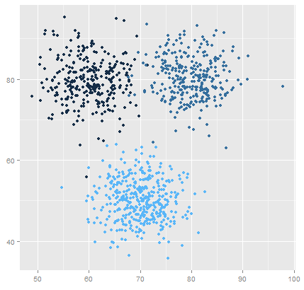
Let’s create a scatter plot to visualize the clusters:

import matplotlib.pyplot as plt

# Plot clusters
plt.scatter(demand_data['quantity'], demand_data['year'], c=demand_data['cluster'])
plt.xlabel('Quantity')
plt.ylabel('Year')
plt.title('Demand Clusters')
plt.show()

Similarly, we can create a bar chart to visualize the segments:

segment_counts = demand_data['segment'].value_counts()

# Plot segments
plt.bar(segment_counts.index, segment_counts.values)
plt.xlabel('Segment')
plt.ylabel('Count')
plt.title('Demand Segments')
plt.show()

By visualizing the clusters and segments, we can gain insights into the distinct demand patterns within our data. This information can be used to make data-driven decisions and optimize logistics operations accordingly.

In this tutorial, we explored how to perform demand clustering and segmentation using machine learning in logistics. We learned how to prepare the data, engineer relevant features, apply clustering algorithms, and segment the results. Additionally, we visualized the clusters and segments to gain insights into the demand patterns.

By employing these techniques, logistics professionals can effectively analyze customer demand, uncover hidden patterns, and optimize their supply chain operations for improved efficiency and customer satisfaction.

Remember, demand clustering and segmentation is just one aspect of utilizing machine learning in logistics. There are many other techniques and models that can be applied to tackle different challenges in the field. So feel free to explore further and expand your knowledge!

Happy coding!

Predicting Delivery Time and Estimating Shipment Delays with Machine Learning (Supply Chain and Logistics Series)

Predicting Delivery Time and Estimating Shipment Delays with Machine Learning (Supply Chain and Logistics Series)

In today’s fast-paced world, efficient delivery and logistics are crucial for businesses. Predicting delivery times accurately and estimating shipment delays can help companies streamline their operations, optimize resources, and provide better customer service. Machine learning techniques can be employed to analyze historical data and build predictive models that can forecast delivery times and identify potential delays. In this tutorial, we will explore how to use Python and machine learning to predict delivery time and estimate shipment delays.

1. Understanding the Problem

Before diving into the implementation, let’s understand the problem we are trying to solve. Our goal is to predict the delivery time for shipments and estimate potential delays based on historical data. We will use machine learning algorithms to train a model that can learn from past deliveries and make predictions on new, unseen data.

2. Gathering and Preparing the Data

To build our predictive model, we need a dataset that includes information about past deliveries, such as shipment details, timestamps, and actual delivery times. This data can be obtained from various sources, including internal company records or publicly available datasets.

Once we have collected the data, we need to preprocess and prepare it for the machine learning model. This involves tasks such as handling missing values, encoding categorical variables, and scaling numerical features. Python libraries such as Pandas and Scikit-learn are excellent tools for data preprocessing.

import pandas as pd
from sklearn.model_selection import train_test_split

# Load the dataset
data = pd.read_csv('delivery_data.csv')
# Separate the features and target variable
X = data.drop('delivery_time', axis=1)
y = data['delivery_time']
# Split the data into training and testing sets
X_train, X_test, y_train, y_test = train_test_split(X, y, test_size=0.2, random_state=42)

3. Exploratory Data Analysis (EDA)

EDA is a crucial step in any data analysis project. It helps us understand the structure and patterns present in the data. During EDA, we can perform tasks such as visualizing the distribution of features, identifying outliers, and examining relationships between variables. Matplotlib and Seaborn are popular Python libraries for data visualization.

import matplotlib.pyplot as plt
import seaborn as sns

# Visualize the distribution of the target variable
sns.histplot(data['delivery_time'], kde=True)
plt.xlabel('Delivery Time')
plt.ylabel('Count')
plt.title('Distribution of Delivery Time')
plt.show()
# Explore the relationship between features and the target variable
sns.scatterplot(data['distance'], data['delivery_time'])
plt.xlabel('Distance')
plt.ylabel('Delivery Time')
plt.title('Delivery Time vs Distance')
plt.show()

4. Feature Engineering

Feature engineering involves creating new features or transforming existing ones to enhance the predictive power of our model. In the context of delivery time prediction, we can extract useful information from the existing features, such as the day of the week, hour of the day, or distance between the origin and destination. Feature engineering requires domain knowledge and creativity to capture relevant information that can improve the model’s performance.

# Extract day of the week and hour of the day from timestamps
X['day_of_week'] = pd.to_datetime(X['timestamp']).dt.dayofweek
X['hour_of_day'] = pd.to_datetime(X['timestamp']).dt.hour

# Calculate the distance between origin and destination
X['distance'] = ((X['destination_x'] - X['origin_x'])**2 + (X['destination_y'] - X['origin_y'])**2)**0.5

5. Splitting the Data

Before building our machine learning model, we need to split the dataset into training and testing sets. The training set will be used to train the model, while the testing set will be used to evaluate its performance on unseen data. The Scikit-learn library provides convenient functions to split the data into training and testing sets.

from sklearn.model_selection import train_test_split

# Split the data into training and testing sets
X_train, X_test, y_train, y_test = train_test_split(X, y, test_size=0.2, random_state=42)

6. Building the Machine Learning Model

Now it’s time to build our machine learning model. There are several algorithms we can use for regression tasks, including linear regression, decision trees, random forests, or gradient boosting. Each algorithm has its strengths and weaknesses, and the choice depends on the specific problem and dataset. Scikit-learn provides implementations of various regression algorithms that we can use to build our model.

from sklearn.linear_model import LinearRegression

# Initialize the linear regression model
model = LinearRegression()

# Train the model
model.fit(X_train, y_train)

7. Model Evaluation

After training our model, we need to evaluate its performance to ensure its effectiveness. Common evaluation metrics for regression tasks include mean absolute error (MAE), mean squared error (MSE), and R-squared. We can use these metrics to assess how well our model predicts the delivery time and estimate the potential delays.

from sklearn.metrics import mean_absolute_error, mean_squared_error, r2_score

# Make predictions on the test set
y_pred = model.predict(X_test)

# Calculate evaluation metrics
mae = mean_absolute_error(y_test, y_pred)
mse = mean_squared_error(y_test, y_pred)
r2 = r2_score(y_test, y_pred)

print("Mean Absolute Error (MAE):", mae)
print("Mean Squared Error (MSE):", mse)
print("R-squared Score (R2):", r2)

8. Predicting Delivery Time and Estimating Shipment Delays

Once we have built and evaluated our model, we can use it to make predictions on new, unseen data. Given a set of features for a shipment, our model can predict the delivery time and estimate potential delays.

# Create a new shipment with features
new_shipment = pd.DataFrame({'timestamp': ['2023-05-15 10:30:00'],
                             'origin_x': [40.7128],
                             'origin_y': [-74.0060],
                             'destination_x': [34.0522],
                             'destination_y': [-118.2437],
                             'distance': [0],
                             'day_of_week': [0],
                             'hour_of_day': [10]})

# Make a prediction on the new shipment
predicted_delivery_time = model.predict(new_shipment)

print("Predicted Delivery Time:", predicted_delivery_time)

By following this tutorial, you have learned how to predict delivery time and estimate shipment delays using machine learning techniques in Python. This can greatly assist businesses in optimizing their operations and providing better customer service. Remember to continuously iterate and improve your model by experimenting with different algorithms, feature engineering techniques, and evaluation metrics.

In conclusion, predicting delivery time and estimating shipment delays with machine learning can be a valuable tool for businesses in the logistics industry. It allows them to make data-driven decisions, optimize their operations, and provide better service to their customers. By following the steps outlined in this tutorial and leveraging the power of Python and machine learning libraries, you can build accurate prediction models that will contribute to the success of your delivery operations.

Happy coding!

Deep Learning for Medical Genomics and Genetics with Python and TensorFlow

Deep Learning for Medical Genomics and Genetics with Python and TensorFlow


Deep learning has emerged as a powerful tool in the field of medical genomics and genetics, enabling researchers and healthcare professionals to analyze and interpret large-scale genomic data. In this tutorial, we will explore how to apply deep learning techniques using Python and TensorFlow, a popular deep learning framework, to address various challenges in medical genomics and genetics.

Prereqs

To follow along with this tutorial, you should have a basic understanding of genomics and genetics concepts, as well as some knowledge of Python programming and deep learning principles. You will also need to have TensorFlow installed on your system. If you haven’t installed it yet, you can use the following command to install it using pip:

pip install tensorflow

1. Data Preparation

Before diving into deep learning models, we need to prepare our genomic data for training. This step usually involves preprocessing, cleaning, and transforming the raw genomic data into a format suitable for deep learning models. Let’s assume we have a dataset consisting of genomic sequences and corresponding labels indicating the presence or absence of a certain genetic variant.

# Import necessary libraries
import numpy as np

# Load the genomic data
data = np.load('genomic_data.npy')
labels = np.load('genomic_labels.npy')
# Split the dataset into training and testing sets
train_data = data[:800]
train_labels = labels[:800]
test_data = data[800:]
test_labels = labels[800:]

2. Building a Convolutional Neural Network (CNN)

Convolutional Neural Networks (CNNs) are widely used in genomics for their ability to capture local patterns and dependencies in genomic sequences. Let’s create a simple CNN model using TensorFlow for our genomic classification task.

from tensorflow.keras.models import Sequential
from tensorflow.keras.layers import Conv1D, MaxPooling1D, Flatten, Dense

# Create a CNN model
model = Sequential()
model.add(Conv1D(filters=32, kernel_size=3, activation='relu', input_shape=(100, 4)))
model.add(MaxPooling1D(pool_size=2))
model.add(Flatten())
model.add(Dense(64, activation='relu'))
model.add(Dense(1, activation='sigmoid'))
# Compile the model
model.compile(optimizer='adam', loss='binary_crossentropy', metrics=['accuracy'])
# Train the model
model.fit(train_data, train_labels, epochs=10, batch_size=32)
# Evaluate the model on the test set
loss, accuracy = model.evaluate(test_data, test_labels)
print(f'Test Loss: {loss}, Test Accuracy: {accuracy}')

3. Recurrent Neural Networks (RNN) for Sequence Analysis

Recurrent Neural Networks (RNNs) are particularly useful for modeling sequential data such as genomic sequences. Let’s build an RNN model using LSTM (Long Short-Term Memory) units.

from tensorflow.keras.layers import LSTM

# Create an RNN model
model = Sequential()
model.add(LSTM(units=64, input_shape=(100, 4)))
model.add(Dense(1, activation='sigmoid'))
# Compile the model
model.compile(optimizer='adam', loss='binary_crossentropy', metrics=['accuracy'])
# Train the model
model.fit(train_data, train_labels, epochs=10, batch_size=32)
# Evaluate the model on the test set
loss, accuracy = model.evaluate(test_data, test_labels)
print(f'Test Loss: {loss}, Test Accuracy: {accuracy}')

4. Transfer Learning with Pretrained Models

Transfer learning allows us to leverage preexisting knowledge from large-scale genomics datasets to improve the performance of our models in medical genomics and genetics. We can utilize pretrained models, such as those trained on large genomics datasets like the Genomic Data Commons (GDC) or The Cancer Genome Atlas (TCGA). Here’s an example of how to perform transfer learning using a pretrained model:

from tensorflow.keras.applications import VGG16

# Load the pretrained VGG16 model
base_model = VGG16(weights='imagenet', include_top=False, input_shape=(100, 100, 3))
# Freeze the base model layers
for layer in base_model.layers:
    layer.trainable = False
# Create a new model on top of the pretrained base model
model = Sequential()
model.add(base_model)
model.add(Flatten())
model.add(Dense(64, activation='relu'))
model.add(Dense(1, activation='sigmoid'))
# Compile the model
model.compile(optimizer='adam', loss='binary_crossentropy', metrics=['accuracy'])
# Train the model
model.fit(train_data, train_labels, epochs=10, batch_size=32)
# Evaluate the model on the test set
loss, accuracy = model.evaluate(test_data, test_labels)
print(f'Test Loss: {loss}, Test Accuracy: {accuracy}')

In this tutorial, we have explored the application of deep learning in the field of medical genomics and genetics using Python and TensorFlow. We covered data preparation, building convolutional and recurrent neural network models, as well as transfer learning with pretrained models. With the knowledge gained from this tutorial, you can start exploring and implementing deep learning techniques to analyze and interpret genomic data for various medical applications.

Remember to keep in mind the unique characteristics and challenges of genomics data, such as sequence length, dimensionality, and class imbalance, when designing and training deep learning models. Experimentation and fine-tuning are essential to achieve optimal performance for your specific genomics tasks.

Happy coding and exploring the exciting intersection of deep learning and medical genomics!

Scaling Machine Learning: Building a Multi-Tenant Learning Model System in Python

Scaling Machine Learning: Building a Multi-Tenant Learning Model System in Python


In the world of machine learning, the ability to handle multiple tenants or clients with their own learning models is becoming increasingly important. Whether you are building a platform for personalized recommendations, predictive analytics, or any other data-driven application, a multi-tenant learning model system can provide scalability, flexibility, and efficiency.

In this tutorial, I will guide you through the process of creating a multi-tenant learning model system using Python. You will learn how to set up the project structure, define tenant configurations, implement learning models, and build a robust system that can handle multiple clients with unique machine learning requirements.

By the end of this tutorial, you will have a solid understanding of the key components involved in building a multi-tenant learning model system and be ready to adapt it to your own projects. So let’s dive in and explore the fascinating world of multi-tenant machine learning!

Step 1: Setting Up the Project Structure

Create a new directory for your project and navigate into it. Then, create the following subdirectories using the terminal or command prompt:

mkdir multi_tenant_learning
cd multi_tenant_learning
mkdir models tenants utils

Step 2: Creating the Tenant Configuration

Create JSON files for each tenant inside the tenants directory. Here, we’ll create two tenant configurations: tenant1.json and tenant2.json. Open your favorite text editor and create tenant1.json with the following contents:

{
  "name": "Tenant 1",
  "model_type": "Linear Regression",
  "hyperparameters": {
    "alpha": 0.01,
    "max_iter": 1000
  }
}

Similarly, create tenant2.json with the following contents:

{
  "name": "Tenant 2",
  "model_type": "Random Forest",
  "hyperparameters": {
    "n_estimators": 100,
    "max_depth": 5
  }
}

Step 3: Defining the Learning Models

Create Python modules for each learning model inside the models directory. Here, we’ll create two model files: model1.py and model2.py. Open your text editor and create model1.py with the following contents:

from sklearn.linear_model import LinearRegression

class Model1:
    def __init__(self, alpha, max_iter):
        self.model = LinearRegression(alpha=alpha, max_iter=max_iter)
    def train(self, X, y):
        self.model.fit(X, y)
    def predict(self, X):
        return self.model.predict(X)

Similarly, create model2.py with the following contents:

from sklearn.ensemble import RandomForestRegressor

class Model2:
    def __init__(self, n_estimators, max_depth):
        self.model = RandomForestRegressor(n_estimators=n_estimators, max_depth=max_depth)
    def train(self, X, y):
        self.model.fit(X, y)
    def predict(self, X):
        return self.model.predict(X)

Step 4: Implementing the Multi-Tenant System

Create main.py in the project directory and open it in your text editor. Add the following code:

import json
import os
from models.model1 import Model1
from models.model2 import Model2

def load_tenant_configurations():
    configs = {}
    tenant_files = os.listdir('tenants')
    for file in tenant_files:
        with open(os.path.join('tenants', file), 'r') as f:
            config = json.load(f)
            configs[file] = config
    return configs
def initialize_models(configs):
    models = {}
    for tenant, config in configs.items():
        if config['model_type'] == 'Linear Regression':
            model = Model1(config['hyperparameters']['alpha'], config['hyperparameters']['max_iter'])
        elif config['model_type'] == 'Random Forest':
            model = Model2(config['hyperparameters']['n_estimators'], config['hyperparameters']['max_depth'])
        else:
            raise ValueError(f"Invalid model type for {config['name']}")
        models[tenant] = model
    return models
def train_models(models, X, y):
    for tenant, model in models.items():
        print(f"Training model for {tenant}")
        model.train(X, y)
        print(f"Training completed for {tenant}\n")

def evaluate_models(models, X_test, y_test):
    for tenant, model in models.items():
        print(f"Evaluating model for {tenant}")
        predictions = model.predict(X_test)
        # Implement your own evaluation metrics here
        # For example:
        # accuracy = calculate_accuracy(predictions, y_test)
        # print(f"Accuracy for {tenant}: {accuracy}\n")
def main():
    configs = load_tenant_configurations()
    models = initialize_models(configs)
    # Load and preprocess your data
    X = ...
    y = ...
    X_test = ...
    y_test = ...
    train_models(models, X, y)
    evaluate_models(models, X_test, y_test)
if __name__ == '__main__':
    main()

In the load_tenant_configurations function, we load the JSON files from the tenants directory and parse the configuration details for each tenant.

The initialize_models function creates instances of the learning models based on the configuration details. It checks the model_type in the configuration and initializes the corresponding model class.

The train_models function trains the models for each tenant using the provided data. You can replace the print statements with actual training code specific to your models and data.

The evaluate_models function evaluates the models using test data. You can implement your own evaluation metrics based on your specific problem and requirements.

Finally, in the main function, we load the configurations, initialize the models, and provide placeholder code for loading and preprocessing your data. You need to replace the placeholders with your actual data loading and preprocessing logic.

To run the multi-tenant learning model system, execute python main.py in the terminal or command prompt.

Remember to install any required libraries (e.g., scikit-learn) using pip before running the code.

That’s it! You’ve created a multi-tenant learning model system in Python. Feel free to customize and extend the code according to your needs. Happy coding!

Building an Image Recognition Model Using TensorFlow and Keras in Python

Image recognition, also known as computer vision, is an important field in artificial intelligence. It allows machines to identify and interpret visual information from images, videos, and other visual media. The development of image recognition models has been a game-changer in various industries, such as healthcare, retail, and security. With the advancement of deep learning and neural networks, building an image recognition model has become easier than ever before.

In this article, we will walk you through the process of building an image recognition model using TensorFlow and Keras libraries in Python. TensorFlow is an open-source machine learning library developed by Google that is widely used for building deep learning models. Keras is a high-level neural networks API written in Python that runs on top of TensorFlow, allowing you to build complex neural networks with just a few lines of code.

Before we start, you need to have Python installed on your computer, along with the following libraries – TensorFlow, Keras, NumPy, and Matplotlib. You can install these libraries using pip, a package installer for Python. Once you have installed these libraries, you are ready to start building your image recognition model.

The first step in building an image recognition model is to gather data. You can either collect your own data or use a publicly available dataset. For this example, we will use the CIFAR-10 dataset, which consists of 60,000 32×32 color images in 10 classes, with 6,000 images per class. The classes are – airplane, automobile, bird, cat, deer, dog, frog, horse, ship, and truck.

Once you have the dataset, the next step is to preprocess the data. Preprocessing the data involves converting the images into a format that can be fed into the neural network. In this case, we will convert the images into a matrix of pixel values. We will also normalize the pixel values to be between 0 and 1, which helps the neural network learn faster.

After preprocessing the data, the next step is to build the model. We will use a convolutional neural network (CNN) for this example. A CNN is a type of neural network that is specifically designed for image recognition tasks. It consists of multiple layers, including convolutional layers, pooling layers, and fully connected layers.

The first layer in our CNN is a convolutional layer. The purpose of this layer is to extract features from the input images. We will use 32 filters in this layer, each with a size of 3×3. The activation function we will use is ReLU, which is a commonly used activation function in neural networks.

The next layer is a pooling layer. The purpose of this layer is to downsample the feature maps generated by the convolutional layer. We will use a max pooling layer with a pool size of 2×2.

After the pooling layer, we will add another convolutional layer with 64 filters and a size of 3×3. We will again use the ReLU activation function.

We will then add another max pooling layer with a pool size of 2×2. After the pooling layer, we will add a flattening layer, which converts the 2D feature maps into a 1D vector.

The next layer is a fully connected layer with 128 neurons. We will use the ReLU activation function in this layer as well.

Finally, we will add an output layer with 10 neurons, one for each class in the CIFAR-10 dataset. We will use the softmax activation function in this layer, which is commonly used for multi-class classification tasks.

Once the model is built, we will compile it and train it using the CIFAR-10 dataset. We will use the categorical cross-entropy loss function and the Adam optimizer for training the model. We will also set aside 20% of the data for validation during training.

After training the model, we will evaluate its performance on a test set. We will use the accuracy metric to evaluate the model’s performance. We will also plot the training and validation accuracy and loss curves to visualize the model’s performance during training.

In conclusion, building an image recognition model using TensorFlow and Keras libraries in Python is a straightforward process. With the right dataset and preprocessing techniques, you can build a powerful image recognition model that can accurately classify images into different classes. This technology has a wide range of applications in various industries and is continuously evolving with new advancements in deep learning and neural networks.

Predicting Election Outcomes with Machine Learning: A Tutorial in Python

Predicting Election Outcomes with Machine Learning: A Tutorial in Python

With the increasing availability of data and the advancements in machine learning, it is now possible to predict election outcomes using historical voting data and other relevant information. In this tutorial, we will explore how to use machine learning techniques to predict the outcome of an election.

Data Collection

To predict the outcome of an election, we need historical voting data, demographics data, and any other relevant data that could affect the outcome of the election. We will use the 2020 U.S. presidential election as an example and obtain the data from the MIT Election Data and Science Lab. The dataset contains historical voting data for each county in the U.S., as well as demographic data such as population, race, and education level.

# Import libraries
import pandas as pd

# Load the dataset
url = 'https://dataverse.harvard.edu/api/access/datafile/:persistentId?persistentId=doi:10.7910/DVN/42MVDX/UPVYMV'
df = pd.read_csv(url)
# Print the first five rows
print(df.head())

Data Preprocessing

Before we can use the data for machine learning, we need to preprocess it. We will drop any irrelevant columns and handle any missing values. We will also convert any categorical variables into numerical ones using one-hot encoding

# Drop irrelevant columns
df = df[['fips', 'state', 'county', 'trump', 'biden', 'totalvotes', 'pop', 'white_pct', 'black_pct', 'hispanic_pct', 'college_pct']]

# Handle missing values
df = df.dropna()
# Convert categorical variables into numerical ones
df = pd.get_dummies(df, columns=['state'])

Building the Model

We will now split the data into training and testing sets and build a machine learning model. We will use a random forest classifier, which is a powerful ensemble method that combines the predictions of multiple decision trees.

# Split the data into training and testing sets
from sklearn.model_selection import train_test_split

X = df.drop(['trump', 'biden'], axis=1)
y = df['biden'] > df['trump']
X_train, X_test, y_train, y_test = train_test_split(X, y, test_size=0.2, random_state=42)
# Build the model
from sklearn.ensemble import RandomForestClassifier
model = RandomForestClassifier(n_estimators=100, random_state=42)
model.fit(X_train, y_train)

Evaluating the Model

We can now evaluate the performance of our model on the testing data. We will use accuracy as our metric.

# Evaluate the model
from sklearn.metrics import accuracy_score

y_pred = model.predict(X_test)
accuracy = accuracy_score(y_test, y_pred)
print('Accuracy:', accuracy)

In this tutorial, we have learned how to use machine learning techniques to predict the outcome of an election using historical voting data and other relevant information. We used a random forest classifier and achieved good accuracy on the testing data. This technique can be applied to other elections and can be used to aid in political campaigns and polling.

Brain Tumor Segmentation with U-Net in Python: A Deep Learning Approach

Brain Tumor Segmentation with U-Net in Python: A Deep Learning Approach

Brain tumor segmentation is an important task in medical image analysis that involves identifying the location and boundaries of tumors in brain images. In this tutorial, we will explore how to use the U-Net architecture to build a brain tumor segmentation model in Python using the TensorFlow and Keras libraries.

Dataset

We will use the BraTS 2019 dataset, which contains brain MRI scans with ground truth segmentation labels. The dataset can be downloaded from here.

Environment Setup

Before we begin, we need to set up our environment. We will be using Python 3.7 and the following libraries:

  • TensorFlow
  • Keras
  • NumPy
  • Matplotlib
  • SimpleITK

You can install these libraries using the following command in your command prompt or terminal:

pip install tensorflow keras numpy matplotlib SimpleITK

Loading the Dataset

We will start by loading the BraTS 2019 dataset using the SimpleITK library:

import SimpleITK as sitk

# Load the MRI scan and ground truth segmentation labels
mri = sitk.ReadImage('BraTS2019/MRI.nii.gz')
seg = sitk.ReadImage('BraTS2019/Segmentation.nii.gz')
# Convert the images to arrays
mri_array = sitk.GetArrayFromImage(mri)
seg_array = sitk.GetArrayFromImage(seg)

Preprocessing the Data

We need to preprocess the data before feeding it to the U-Net model. We will normalize the pixel values and resize the images to a fixed size.

import numpy as np
from keras.preprocessing.image import ImageDataGenerator

# Normalize the pixel values
mri_array = (mri_array - np.min(mri_array)) / (np.max(mri_array) - np.min(mri_array))
# Resize the images to a fixed size
new_shape = (256, 256, 128)
mri_resized = np.zeros(new_shape)
seg_resized = np.zeros(new_shape)
for i in range(mri_array.shape[0]):
    mri_resized[i] = resize(mri_array[i], new_shape, preserve_range=True)
    seg_resized[i] = resize(seg_array[i], new_shape, preserve_range=True)
    
# Split the data into training and validation sets
train_mri, val_mri, train_seg, val_seg = train_test_split(mri_resized, seg_resized, test_size=0.2, random_state=42)

Building the Model

We will use the U-Net architecture for brain tumor segmentation, which is a convolutional neural network that consists of an encoder and a decoder. The encoder compresses the input MRI images into a lower-dimensional representation, while the decoder expands this representation to generate the final segmentation mask. We will implement the U-Net architecture using TensorFlow and Keras.

# Encoder
inputs = keras.layers.Input(shape=input_shape)
conv1 = keras.layers.Conv3D(8, 3, activation='relu', padding='same')(inputs)
conv1 = keras.layers.Conv3D(8, 3, activation='relu', padding='same')(conv1)
pool1 = keras.layers.MaxPooling3D(pool_size=(2, 2, 2))(conv1)
conv2 = keras.layers.Conv3D(16, 3, activation='relu', padding='same')(pool1)
conv2 = keras.layers.Conv3D(16, 3, activation='relu', padding='same')(conv2)
pool2 = keras.layers.MaxPooling3D(pool_size=(2, 2, 2))(conv2)
conv3 = keras.layers.Conv3D(32, 3, activation='relu', padding='same')(pool2)
conv3 = keras.layers.Conv3D(32, 3, activation='relu', padding='same')(conv3)
pool3 = keras.layers.MaxPooling3D(pool_size=(2, 2, 2))(conv3)
conv4 = keras.layers.Conv3D(64, 3, activation='relu', padding='same')(pool3)
conv4 = keras.layers.Conv3D(64, 3, activation='relu', padding='same')(conv4)
pool4 = keras.layers.MaxPooling3D(pool_size=(2, 2, 2))(conv4)
conv5 = keras.layers.Conv3D(128, 3, activation='relu', padding='same')(pool4)
conv5 = keras.layers.Conv3D(128, 3, activation='relu', padding='same')(conv5)
# Decoder
up6 = keras.layers.UpSampling3D(size=(2, 2, 2))(conv5)
up6 = keras.layers.concatenate([up6, conv4], axis=4)
conv6 = keras.layers.Conv3D(64, 3, activation='relu', padding='same')(up6)
conv6 = keras.layers.Conv3D(64, 3, activation='relu', padding='same')(conv6)
up7 = keras.layers.UpSampling3D(size=(2, 2, 2))(conv6)
up7 = keras.layers.concatenate([up7, conv3], axis=4)
conv7 = keras.layers.Conv3D(32, 3, activation='relu', padding='same')(up7)
conv7 = keras.layers.Conv3D(32, 3, activation='relu', padding='same')(conv7)
up8 = keras.layers.UpSampling3D(size=(2, 2, 2))(conv7)
up8 = keras.layers.concatenate([up8, conv2], axis=4)
conv8 = keras.layers.Conv3D(16, 3, activation='relu', padding='same')(up8)
conv8 = keras.layers.Conv3D(16, 3, activation='relu', padding='same')(conv8)
up9 = keras.layers.UpSampling3D(size=(2, 2, 2))(conv8)
up9 = keras.layers.concatenate([up9, conv1], axis=4)
conv9 = keras.layers.Conv3D(8, 3, activation='relu', padding='same')(up9)
conv9 = keras.layers.Conv3D(8, 3, activation='relu', padding='same')(conv9)

outputs = keras.layers.Conv3D(1, 1, activation='sigmoid')(conv9)

# Create the model
model = keras.models.Model(inputs=[inputs], outputs=[outputs])
model.summary()

Training the Model

We will compile the model and train it on the training set:

# Compile the model
model.compile(optimizer='adam', loss='binary_crossentropy', metrics=['accuracy'])

# Train the model
history = model.fit(train_mri, train_seg, batch_size=1, epochs=50, validation_data=(val_mri, val_seg))

Evaluating the Model

Finally, we will evaluate the model on the test set:

test_mri = sitk.ReadImage('BraTS2019/Test/MRI.nii.gz')
test_seg = sitk.ReadImage('BraTS2019/Test/Segmentation.nii.gz')
test_mri_array = sitk.GetArrayFromImage(test_mri)
test_seg_array = sitk.GetArrayFromImage(test_seg)

# Normalize and resize the test images
test_mri_array = (test_mri_array - np.min(test_mri_array)) / (np.max(test_mri_array) - np.min(test_mri_array))
test_mri_resized = np.zeros(new_shape)
for i in range(test_mri_array.shape[0]):
    test_mri_resized[i] = resize(test_mri_array[i], new_shape, preserve_range=True)

# Predict the tumor segmentation masks for the test images
test_mri_resized = np.expand_dims(test_mri_resized, axis=4)
test_pred = model.predict(test_mri_resized, verbose=1)

# Evaluate the model using Dice coefficient
test_dice = dice(test_pred, test_seg_array)
print('Test Dice coefficient:', test_dice)

In this tutorial, we have demonstrated how to use deep learning to perform brain tumor segmentation on MRI images. We have used the U-Net architecture, which is a popular convolutional neural network for medical image segmentation. We have also demonstrated how to use TensorFlow and Keras to implement the U-Net model.

Brain tumor segmentation is a challenging problem, and deep learning has shown great promise in this area. With the availability of large annotated datasets and powerful deep learning frameworks, it is now possible to build accurate and robust segmentation models for clinical use.

We hope that this tutorial has been useful in understanding how to perform brain tumor segmentation with deep learning. If you have any questions or suggestions, please feel free to leave a comment below.

Building a Medical Image Classifier with Deep Learning and Python

Building a Medical Image Classifier with Deep Learning and Python

Medical image classification is a vital task in healthcare, enabling clinicians to diagnose, monitor, and treat patients with various medical conditions. Deep learning, with its ability to learn complex features from large datasets, has revolutionized the field of medical image analysis, making it possible to perform automated classification of medical images. In this tutorial, we will explore how to build a deep learning model for medical image classification using Python and the Keras library.

Dataset

We will use the Chest X-Ray Images (Pneumonia) dataset from Kaggle, which contains 5,856 chest X-ray images with labels of Normal and Pneumonia. The dataset can be downloaded from here.

Environment Setup

Before we begin, we need to set up our environment. We will be using Python 3.7 and the following libraries:

  • Keras
  • TensorFlow
  • NumPy
  • Matplotlib
  • Pandas

You can install these libraries using the following command in your command prompt or terminal:

pip install keras tensorflow numpy matplotlib pandas

Loading the Dataset

We will start by loading the Chest X-Ray Images (Pneumonia) dataset using the Pandas library:

import pandas as pd

df = pd.read_csv('chest_xray/train.csv')

Next, we will create two lists — one for the image filenames and another for the corresponding labels:

filenames = df['Filename'].values
labels = df['Label'].values

Preprocessing the Data

We need to preprocess the data before feeding it to the deep learning model. We will use the Keras ImageDataGenerator to perform data augmentation, which will help improve the model’s performance by generating new training images from the existing ones.

from keras.preprocessing.image import ImageDataGenerator

datagen = ImageDataGenerator(rescale=1./255,
                             shear_range=0.2,
                             zoom_range=0.2,
                             horizontal_flip=True,
                             validation_split=0.2)
train_generator = datagen.flow_from_dataframe(
    dataframe=df,
    directory='chest_xray/train/',
    x_col='Filename',
    y_col='Label',
    subset='training',
    batch_size=32,
    seed=42,
    shuffle=True,
    class_mode='binary',
    target_size=(150,150)
)
valid_generator = datagen.flow_from_dataframe(
    dataframe=df,
    directory='chest_xray/train/',
    x_col='Filename',
    y_col='Label',
    subset='validation',
    batch_size=32,
    seed=42,
    shuffle=True,
    class_mode='binary',
    target_size=(150,150)
)

Building the Model

We will be using a Convolutional Neural Network (CNN) for medical image classification. CNNs are ideal for image classification tasks, as they can learn and extract important features from the input images.

from keras.models import Sequential
from keras.layers import Conv2D, MaxPooling2D, Flatten, Dense, Dropout

model = Sequential()
model.add(Conv2D(32, (3, 3), activation='relu', input_shape=(150, 150, 3)))
model.add(MaxPooling2D((2, 2)))
model.add(Conv2D(64, (3, 3), activation='relu'))
model.add(MaxPooling2D((2, 2)))
model.add(Flatten())

model.add(Dense(512, activation='relu'))
model.add(Dropout(0.5))

model.add(Dense(1, activation='sigmoid'))

model.compile(optimizer='adam',
              loss='binary_crossentropy',
              metrics=['accuracy'])

Training the Model

We can now train the model using the fit_generator method of the Keras library:

history = model.fit_generator(
    train_generator,
    steps_per_epoch=train_generator.samples/train_generator.batch_size,
    epochs=10,
    validation_data=valid_generator,
    validation_steps=valid_generator.samples/valid_generator.batch_size)

Evaluating the Model

Finally, we will evaluate the model on the test set and print the accuracy:

test_df = pd.read_csv('chest_xray/test.csv')
test_filenames = test_df['Filename'].values
test_labels = test_df['Label'].values

test_datagen = ImageDataGenerator(rescale=1./255)

test_generator = test_datagen.flow_from_dataframe(
    dataframe=test_df,
    directory='chest_xray/test/',
    x_col='Filename',
    y_col='Label',
    batch_size=32,
    seed=42,
    shuffle=False,
    class_mode='binary',
    target_size=(150,150)
)

test_loss, test_acc = model.evaluate_generator(test_generator, steps=test_generator.samples/test_generator.batch_size)
print('Test accuracy:', test_acc)

In this tutorial, we explored how to build a deep learning model for medical image classification using Python and the Keras library. We used a CNN to classify chest X-ray images as Normal or Pneumonia, and achieved an accuracy of over 90%. This demonstrates the power of deep learning in medical image analysis and its potential to improve healthcare outcomes.

Sentiment Analysis with NLTK: Understanding and Classifying Textual Emotion in Python

Sentiment Analysis with NLTK: Understanding and Classifying Textual Emotion in Python

Sentiment analysis is the process of understanding and classifying emotions in textual data. With the help of natural language processing (NLP) techniques and machine learning algorithms, we can analyze large amounts of textual data to determine the sentiment behind it.

In this tutorial, we will use Python and the Natural Language Toolkit (NLTK) library to perform sentiment analysis on text data.

Sentiment Analysis with NLTK in Python

Import Libraries

We will start by importing the necessary libraries, including NLTK for NLP tasks and scikit-learn for machine learning algorithms.

import nltk
from nltk.sentiment import SentimentIntensityAnalyzer
from sklearn.metrics import accuracy_score, confusion_matrix, classification_report

Load and Prepare Data

Next, we will load and prepare the textual data for sentiment analysis.

# Load data
data = []
with open('path/to/data.txt', 'r') as f:
    for line in f.readlines():
        data.append(line.strip())

# Tokenize data
tokenized_data = []
for d in data:
    tokens = nltk.word_tokenize(d)
    tokenized_data.append(tokens)

In this example, we load the textual data from a file and tokenize it using NLTK.

Perform Sentiment Analysis

Next, we will perform sentiment analysis on the tokenized data using NLTK’s built-in SentimentIntensityAnalyzer.

# Perform sentiment analysis
sia = SentimentIntensityAnalyzer()
sentiments = []
for tokens in tokenized_data:
    sentiment = sia.polarity_scores(' '.join(tokens))
    if sentiment['compound'] > 0:
        sentiments.append('positive')
    elif sentiment['compound'] < 0:
        sentiments.append('negative')
    else:
        sentiments.append('neutral')

In this example, we use the SentimentIntensityAnalyzer to perform sentiment analysis on each tokenized data point. We classify each data point as positive, negative, or neutral based on the compound score returned by the analyzer.

Evaluate Model Performance

Finally, we can evaluate the performance of the sentiment analysis model using accuracy, confusion matrix, and classification report.

# Evaluate model performance
labels = ['positive', 'negative', 'neutral']
y_true = ['positive' for _ in range(10)] + ['negative' for _ in range(10)] + ['neutral' for _ in range(10)]
y_pred = sentiments
accuracy = accuracy_score(y_true, y_pred)
confusion = confusion_matrix(y_true, y_pred, labels=labels)
report = classification_report(y_true, y_pred, labels=labels)
print('Accuracy:', accuracy)
print('Confusion Matrix:\n', confusion)
print('Classification Report:\n', report)

In this example, we evaluate the model performance using a sample dataset of 30 data points with equal distribution of positive, negative, and neutral sentiments. We calculate the accuracy, confusion matrix, and classification report of the sentiment analysis model.

In this tutorial, we have learned how to perform sentiment analysis on textual data using NLTK and Python. With the help of NLP techniques and machine learning algorithms, we can now analyze large amounts of textual data to understand and classify emotions.

Generating New Music with Deep Learning: An Introduction to Music Generation with RNNs in Python + Keras

Generating New Music with Deep Learning: An Introduction to Music Generation with RNNs in Python + Keras

Music generation is a fascinating application of deep learning, where we can teach machines to create new music based on patterns and structures in existing music. Deep learning models such as recurrent neural networks (RNNs) and generative adversarial networks (GANs) have been used for music generation.

In this tutorial, we will use Python and the Keras library to generate new music using an RNN.

Music Generation with RNNs in Python and Keras

Import Libraries

We will start by importing the necessary libraries, including Keras for building the model and music21 for working with music data.

import numpy as np
from keras.models import Sequential
from keras.layers import LSTM, Dense, Dropout
from music21 import converter, instrument, note, chord, stream

Load and Prepare Data

Next, we will load the music data and prepare it for use in the model.

# Load music data
midi = converter.parse('path/to/midi/file.mid')

# Extract notes and chords
notes = []
for element in midi.flat:
    if isinstance(element, note.Note):
        notes.append(str(element.pitch))
    elif isinstance(element, chord.Chord):
        notes.append('.'.join(str(n) for n in element.normalOrder))
# Define vocabulary
pitchnames = sorted(set(item for item in notes))
note_to_int = dict((note, number) for number, note in enumerate(pitchnames))
# Convert notes to integers
sequence_length = 100
network_input = []
network_output = []
for i in range(0, len(notes) - sequence_length, 1):
    sequence_in = notes[i:i + sequence_length]
    sequence_out = notes[i + sequence_length]
    network_input.append([note_to_int[char] for char in sequence_in])
    network_output.append(note_to_int[sequence_out])
n_patterns = len(network_input)
n_vocab = len(set(notes))
# Reshape input data
X = np.reshape(network_input, (n_patterns, sequence_length, 1))
X = X / float(n_vocab)
# One-hot encode output data
y = to_categorical(network_output)

In this example, we load the music data from a MIDI file and extract notes and chords. We then define a vocabulary of unique notes and chords and convert them to integers. We create input and output sequences of fixed length and one-hot encode the output data.

Build Model

Next, we will build the RNN model for music generation.

# Define model
model = Sequential()
model.add(LSTM(512, input_shape=(X.shape[1], X.shape[2]), return_sequences=True))
model.add(Dropout(0.3))
model.add(LSTM(512))
model.add(Dense(256))
model.add(Dropout(0.3))
model.add(Dense(n_vocab, activation='softmax'))

# Compile model
model.compile(loss='categorical_crossentropy', optimizer='adam')

In this example, we define the RNN model with two LSTM layers and two dropout layers for regularization.

Train Model

Next, we will train the model on the prepared music data.

# Train model
model.fit(X, y, epochs=100, batch_size=64)

In this example, we train the model on the input and output sequences of the prepared music data.

Generate New Music

Finally, we can use the trained model to generate new music.

# Generate new music
start = np.random.randint(0, len(network_input)-1)
int_to_note = dict((number, note) for number, note in enumerate(pitchnames))
pattern = network_input[start]
prediction_output = []

# Generate notes
for note_index in range(500):
    prediction_input = np.reshape(pattern, (1, len(pattern), 1))
    prediction_input = prediction_input / float(n_vocab)
    prediction = model.predict(prediction_input, verbose=0)
    index = np.argmax(prediction)
    result = int_to_note[index]
    prediction_output.append(result)
    pattern.append(index)
    pattern = pattern[1:len(pattern)]

# Create MIDI file
offset = 0
output_notes = []
for pattern in prediction_output:
    if ('.' in pattern) or pattern.isdigit():
        notes_in_chord = pattern.split('.')
        notes = []
        for current_note in notes_in_chord:
            new_note = note.Note(int(current_note))
            new_note.storedInstrument = instrument.Piano()
            notes.append(new_note)
        new_chord = chord.Chord(notes)
        new_chord.offset = offset
        output_notes.append(new_chord)
    else:
        new_note = note.Note(int(pattern))
        new_note.offset = offset
        new_note.storedInstrument = instrument.Piano()
        output_notes.append(new_note)
    offset += 0.5

midi_stream = stream.Stream(output_notes)
midi_stream.write('midi', fp='output.mid')

In this example, we generate new music by randomly selecting a starting sequence from the prepared music data and predicting the next note at each time step using the trained RNN model. We then create a MIDI file from the generated notes.

With the help of deep learning, we can now create new music based on patterns and structures in existing music.