Posts Tagged

keras

Building an Image Recognition Model Using TensorFlow and Keras in Python

Image recognition, also known as computer vision, is an important field in artificial intelligence. It allows machines to identify and interpret visual information from images, videos, and other visual media. The development of image recognition models has been a game-changer in various industries, such as healthcare, retail, and security. With the advancement of deep learning and neural networks, building an image recognition model has become easier than ever before.

In this article, we will walk you through the process of building an image recognition model using TensorFlow and Keras libraries in Python. TensorFlow is an open-source machine learning library developed by Google that is widely used for building deep learning models. Keras is a high-level neural networks API written in Python that runs on top of TensorFlow, allowing you to build complex neural networks with just a few lines of code.

Before we start, you need to have Python installed on your computer, along with the following libraries – TensorFlow, Keras, NumPy, and Matplotlib. You can install these libraries using pip, a package installer for Python. Once you have installed these libraries, you are ready to start building your image recognition model.

The first step in building an image recognition model is to gather data. You can either collect your own data or use a publicly available dataset. For this example, we will use the CIFAR-10 dataset, which consists of 60,000 32×32 color images in 10 classes, with 6,000 images per class. The classes are – airplane, automobile, bird, cat, deer, dog, frog, horse, ship, and truck.

Once you have the dataset, the next step is to preprocess the data. Preprocessing the data involves converting the images into a format that can be fed into the neural network. In this case, we will convert the images into a matrix of pixel values. We will also normalize the pixel values to be between 0 and 1, which helps the neural network learn faster.

After preprocessing the data, the next step is to build the model. We will use a convolutional neural network (CNN) for this example. A CNN is a type of neural network that is specifically designed for image recognition tasks. It consists of multiple layers, including convolutional layers, pooling layers, and fully connected layers.

The first layer in our CNN is a convolutional layer. The purpose of this layer is to extract features from the input images. We will use 32 filters in this layer, each with a size of 3×3. The activation function we will use is ReLU, which is a commonly used activation function in neural networks.

The next layer is a pooling layer. The purpose of this layer is to downsample the feature maps generated by the convolutional layer. We will use a max pooling layer with a pool size of 2×2.

After the pooling layer, we will add another convolutional layer with 64 filters and a size of 3×3. We will again use the ReLU activation function.

We will then add another max pooling layer with a pool size of 2×2. After the pooling layer, we will add a flattening layer, which converts the 2D feature maps into a 1D vector.

The next layer is a fully connected layer with 128 neurons. We will use the ReLU activation function in this layer as well.

Finally, we will add an output layer with 10 neurons, one for each class in the CIFAR-10 dataset. We will use the softmax activation function in this layer, which is commonly used for multi-class classification tasks.

Once the model is built, we will compile it and train it using the CIFAR-10 dataset. We will use the categorical cross-entropy loss function and the Adam optimizer for training the model. We will also set aside 20% of the data for validation during training.

After training the model, we will evaluate its performance on a test set. We will use the accuracy metric to evaluate the model’s performance. We will also plot the training and validation accuracy and loss curves to visualize the model’s performance during training.

In conclusion, building an image recognition model using TensorFlow and Keras libraries in Python is a straightforward process. With the right dataset and preprocessing techniques, you can build a powerful image recognition model that can accurately classify images into different classes. This technology has a wide range of applications in various industries and is continuously evolving with new advancements in deep learning and neural networks.

Building a Medical Image Classifier with Deep Learning and Python

Building a Medical Image Classifier with Deep Learning and Python

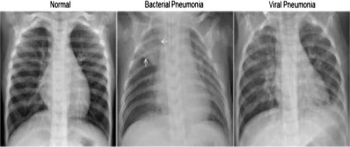
Medical image classification is a vital task in healthcare, enabling clinicians to diagnose, monitor, and treat patients with various medical conditions. Deep learning, with its ability to learn complex features from large datasets, has revolutionized the field of medical image analysis, making it possible to perform automated classification of medical images. In this tutorial, we will explore how to build a deep learning model for medical image classification using Python and the Keras library.

Dataset

We will use the Chest X-Ray Images (Pneumonia) dataset from Kaggle, which contains 5,856 chest X-ray images with labels of Normal and Pneumonia. The dataset can be downloaded from here.

Environment Setup

Before we begin, we need to set up our environment. We will be using Python 3.7 and the following libraries:

  • Keras
  • TensorFlow
  • NumPy
  • Matplotlib
  • Pandas

You can install these libraries using the following command in your command prompt or terminal:

pip install keras tensorflow numpy matplotlib pandas

Loading the Dataset

We will start by loading the Chest X-Ray Images (Pneumonia) dataset using the Pandas library:

import pandas as pd

df = pd.read_csv('chest_xray/train.csv')

Next, we will create two lists — one for the image filenames and another for the corresponding labels:

filenames = df['Filename'].values
labels = df['Label'].values

Preprocessing the Data

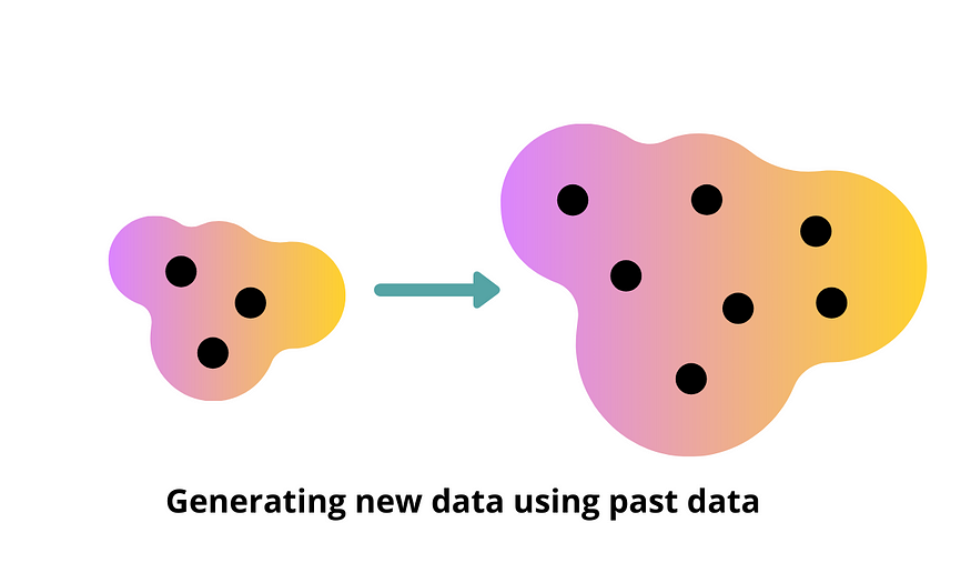
We need to preprocess the data before feeding it to the deep learning model. We will use the Keras ImageDataGenerator to perform data augmentation, which will help improve the model’s performance by generating new training images from the existing ones.

from keras.preprocessing.image import ImageDataGenerator

datagen = ImageDataGenerator(rescale=1./255,
                             shear_range=0.2,
                             zoom_range=0.2,
                             horizontal_flip=True,
                             validation_split=0.2)
train_generator = datagen.flow_from_dataframe(
    dataframe=df,
    directory='chest_xray/train/',
    x_col='Filename',
    y_col='Label',
    subset='training',
    batch_size=32,
    seed=42,
    shuffle=True,
    class_mode='binary',
    target_size=(150,150)
)
valid_generator = datagen.flow_from_dataframe(
    dataframe=df,
    directory='chest_xray/train/',
    x_col='Filename',
    y_col='Label',
    subset='validation',
    batch_size=32,
    seed=42,
    shuffle=True,
    class_mode='binary',
    target_size=(150,150)
)

Building the Model

We will be using a Convolutional Neural Network (CNN) for medical image classification. CNNs are ideal for image classification tasks, as they can learn and extract important features from the input images.

from keras.models import Sequential
from keras.layers import Conv2D, MaxPooling2D, Flatten, Dense, Dropout

model = Sequential()
model.add(Conv2D(32, (3, 3), activation='relu', input_shape=(150, 150, 3)))
model.add(MaxPooling2D((2, 2)))
model.add(Conv2D(64, (3, 3), activation='relu'))
model.add(MaxPooling2D((2, 2)))
model.add(Flatten())

model.add(Dense(512, activation='relu'))
model.add(Dropout(0.5))

model.add(Dense(1, activation='sigmoid'))

model.compile(optimizer='adam',
              loss='binary_crossentropy',
              metrics=['accuracy'])

Training the Model

We can now train the model using the fit_generator method of the Keras library:

history = model.fit_generator(
    train_generator,
    steps_per_epoch=train_generator.samples/train_generator.batch_size,
    epochs=10,
    validation_data=valid_generator,
    validation_steps=valid_generator.samples/valid_generator.batch_size)

Evaluating the Model

Finally, we will evaluate the model on the test set and print the accuracy:

test_df = pd.read_csv('chest_xray/test.csv')
test_filenames = test_df['Filename'].values
test_labels = test_df['Label'].values

test_datagen = ImageDataGenerator(rescale=1./255)

test_generator = test_datagen.flow_from_dataframe(
    dataframe=test_df,
    directory='chest_xray/test/',
    x_col='Filename',
    y_col='Label',
    batch_size=32,
    seed=42,
    shuffle=False,
    class_mode='binary',
    target_size=(150,150)
)

test_loss, test_acc = model.evaluate_generator(test_generator, steps=test_generator.samples/test_generator.batch_size)
print('Test accuracy:', test_acc)

In this tutorial, we explored how to build a deep learning model for medical image classification using Python and the Keras library. We used a CNN to classify chest X-ray images as Normal or Pneumonia, and achieved an accuracy of over 90%. This demonstrates the power of deep learning in medical image analysis and its potential to improve healthcare outcomes.

Generating New Music with Deep Learning: An Introduction to Music Generation with RNNs in Python + Keras

Generating New Music with Deep Learning: An Introduction to Music Generation with RNNs in Python + Keras

Music generation is a fascinating application of deep learning, where we can teach machines to create new music based on patterns and structures in existing music. Deep learning models such as recurrent neural networks (RNNs) and generative adversarial networks (GANs) have been used for music generation.

In this tutorial, we will use Python and the Keras library to generate new music using an RNN.

Music Generation with RNNs in Python and Keras

Import Libraries

We will start by importing the necessary libraries, including Keras for building the model and music21 for working with music data.

import numpy as np
from keras.models import Sequential
from keras.layers import LSTM, Dense, Dropout
from music21 import converter, instrument, note, chord, stream

Load and Prepare Data

Next, we will load the music data and prepare it for use in the model.

# Load music data
midi = converter.parse('path/to/midi/file.mid')

# Extract notes and chords
notes = []
for element in midi.flat:
    if isinstance(element, note.Note):
        notes.append(str(element.pitch))
    elif isinstance(element, chord.Chord):
        notes.append('.'.join(str(n) for n in element.normalOrder))
# Define vocabulary
pitchnames = sorted(set(item for item in notes))
note_to_int = dict((note, number) for number, note in enumerate(pitchnames))
# Convert notes to integers
sequence_length = 100
network_input = []
network_output = []
for i in range(0, len(notes) - sequence_length, 1):
    sequence_in = notes[i:i + sequence_length]
    sequence_out = notes[i + sequence_length]
    network_input.append([note_to_int[char] for char in sequence_in])
    network_output.append(note_to_int[sequence_out])
n_patterns = len(network_input)
n_vocab = len(set(notes))
# Reshape input data
X = np.reshape(network_input, (n_patterns, sequence_length, 1))
X = X / float(n_vocab)
# One-hot encode output data
y = to_categorical(network_output)

In this example, we load the music data from a MIDI file and extract notes and chords. We then define a vocabulary of unique notes and chords and convert them to integers. We create input and output sequences of fixed length and one-hot encode the output data.

Build Model

Next, we will build the RNN model for music generation.

# Define model
model = Sequential()
model.add(LSTM(512, input_shape=(X.shape[1], X.shape[2]), return_sequences=True))
model.add(Dropout(0.3))
model.add(LSTM(512))
model.add(Dense(256))
model.add(Dropout(0.3))
model.add(Dense(n_vocab, activation='softmax'))

# Compile model
model.compile(loss='categorical_crossentropy', optimizer='adam')

In this example, we define the RNN model with two LSTM layers and two dropout layers for regularization.

Train Model

Next, we will train the model on the prepared music data.

# Train model
model.fit(X, y, epochs=100, batch_size=64)

In this example, we train the model on the input and output sequences of the prepared music data.

Generate New Music

Finally, we can use the trained model to generate new music.

# Generate new music
start = np.random.randint(0, len(network_input)-1)
int_to_note = dict((number, note) for number, note in enumerate(pitchnames))
pattern = network_input[start]
prediction_output = []

# Generate notes
for note_index in range(500):
    prediction_input = np.reshape(pattern, (1, len(pattern), 1))
    prediction_input = prediction_input / float(n_vocab)
    prediction = model.predict(prediction_input, verbose=0)
    index = np.argmax(prediction)
    result = int_to_note[index]
    prediction_output.append(result)
    pattern.append(index)
    pattern = pattern[1:len(pattern)]

# Create MIDI file
offset = 0
output_notes = []
for pattern in prediction_output:
    if ('.' in pattern) or pattern.isdigit():
        notes_in_chord = pattern.split('.')
        notes = []
        for current_note in notes_in_chord:
            new_note = note.Note(int(current_note))
            new_note.storedInstrument = instrument.Piano()
            notes.append(new_note)
        new_chord = chord.Chord(notes)
        new_chord.offset = offset
        output_notes.append(new_chord)
    else:
        new_note = note.Note(int(pattern))
        new_note.offset = offset
        new_note.storedInstrument = instrument.Piano()
        output_notes.append(new_note)
    offset += 0.5

midi_stream = stream.Stream(output_notes)
midi_stream.write('midi', fp='output.mid')

In this example, we generate new music by randomly selecting a starting sequence from the prepared music data and predicting the next note at each time step using the trained RNN model. We then create a MIDI file from the generated notes.

With the help of deep learning, we can now create new music based on patterns and structures in existing music.

Optimizing Model Performance: A Guide to Hyperparameter Tuning in Python with Keras

Optimizing Model Performance: A Guide to Hyperparameter Tuning in Python with Keras

Hyperparameter tuning is the process of selecting the best set of hyperparameters for a machine learning model to optimize its performance. Hyperparameters are values that cannot be learned from the data, but are set by the user before training the model. Examples of hyperparameters include learning rate, batch size, number of hidden layers, and number of neurons in each hidden layer.

Optimizing hyperparameters is important because it can significantly improve the performance of a machine learning model. However, it can be a time-consuming and computationally expensive process.

In this tutorial, we will use Python to demonstrate how to perform hyperparameter tuning using the Keras library.

Hyperparameter Tuning in Python with Keras

Import Libraries

We will start by importing the necessary libraries, including Keras for building the model and scikit-learn for hyperparameter tuning.

import numpy as np
from keras.datasets import mnist
from keras.models import Sequential
from keras.layers import Dense, Dropout
from keras.utils import to_categorical
from keras.optimizers import Adam
from sklearn.model_selection import RandomizedSearchCV

Load Data

Next, we will load the MNIST dataset for training and testing the model.

# Load data
(x_train, y_train), (x_test, y_test) = mnist.load_data()

# Normalize data
x_train = x_train.astype('float32') / 255.
x_test = x_test.astype('float32') / 255.
# Flatten data
x_train = x_train.reshape((len(x_train), np.prod(x_train.shape[1:])))
x_test = x_test.reshape((len(x_test), np.prod(x_test.shape[1:])))
# One-hot encode labels
y_train = to_categorical(y_train)
y_test = to_categorical(y_test)

In this example, we load the MNIST dataset and normalize and flatten the data. We also one-hot encode the labels.

Build Model

Next, we will build the model.

# Define model
def build_model(learning_rate=0.01, dropout_rate=0.0, neurons=64):

model = Sequential()
    model.add(Dense(neurons, activation='relu', input_shape=(784,)))
    model.add(Dropout(dropout_rate))
    model.add(Dense(neurons, activation='relu'))
    model.add(Dropout(dropout_rate))
    model.add(Dense(10, activation='softmax'))
    optimizer = Adam(lr=learning_rate)
    model.compile(loss='categorical_crossentropy', optimizer=optimizer, metrics=['accuracy'])
    return model

In this example, we define the model with three layers, including two hidden layers with a user-defined number of neurons and a dropout layer for regularization.

Perform Hyperparameter Tuning

Next, we will perform hyperparameter tuning using scikit-learn’s RandomizedSearchCV function.

# Define hyperparameters
params = {
    'learning_rate': [0.01, 0.001, 0.0001],
    'dropout_rate': [0.0, 0.1, 0.2],
    'neurons': [32, 64, 128],
    'batch_size': [32, 64, 128]
}

# Create model
model = build_model()
# Perform hyperparameter tuning
random_search = RandomizedSearchCV(model, param_distributions=params, cv=3)
random_search.fit(x_train, y_train)
# Print best hyperparameters
print(random_search.best_params_)

In this example, we define a dictionary of hyperparameters and their values to be tuned. We then create the model and perform hyperparameter tuning using RandomizedSearchCV with a 3-fold cross-validation. Finally, we print the best hyperparameters found during the tuning process.

Evaluate Model

Once we have found the best hyperparameters, we can build the final model with those hyperparameters and evaluate its performance on the testing data.

# Build final model with best hyperparameters
best_learning_rate = random_search.best_params_['learning_rate']
best_dropout_rate = random_search.best_params_['dropout_rate']
best_neurons = random_search.best_params_['neurons']
model = build_model(learning_rate=best_learning_rate, dropout_rate=best_dropout_rate, neurons=best_neurons)

# Train model
model.fit(x_train, y_train, batch_size=128, epochs=10, validation_data=(x_test, y_test))
# Evaluate model on testing data
score = model.evaluate(x_test, y_test, verbose=0)
print('Test loss:', score[0])
print('Test accuracy:', score[1])

In this example, we build the final model with the best hyperparameters found during hyperparameter tuning. We then train the model and evaluate its performance on the testing data.

In this tutorial, we covered the basics of hyperparameter tuning and how to perform it using Python with Keras and scikit-learn. By tuning the hyperparameters, we can significantly improve the performance of a machine learning model. I hope you found this tutorial useful in understanding how to optimize model performance through hyperparameter tuning.

Creating New Data with Generative Models in Python

Creating New Data with Generative Models in Python

Generative models are a type of machine learning model that can create new data based on the patterns and structure of existing data. Generative models learn the underlying distribution of the data and can generate new samples that are similar to the original data. Generative models are useful in scenarios where the data is limited or where the generation of new data is required.

Generative Models in Python

Python is a popular language for machine learning, and several libraries support generative models. In this tutorial, we will use the Keras library to build and train a generative model in Python.

Import Libraries

We will start by importing the necessary libraries, including Keras for generative models, and NumPy and Matplotlib for data processing and visualization.

import numpy as np
import matplotlib.pyplot as plt
from keras.layers import Input, Dense, Reshape, Flatten
from keras.layers.advanced_activations import LeakyReLU
from keras.models import Sequential, Model
from keras.optimizers import Adam

Load Data

Next, we will load the data to train the generative model.

# Load data
(x_train, y_train), (_, _) = tf.keras.datasets.mnist.load_data()

# Normalize data
x_train = x_train / 255.0
# Flatten data
x_train = x_train.reshape(x_train.shape[0], -1)

In this example, we load the MNIST dataset and normalize and flatten the data.

Build Generative Model

Next, we will build the generative model.

# Build generative model
def build_generator():

# Define input layer
    input_layer = Input(shape=(100,))
    # Define hidden layers
    hidden_layer_1 = Dense(128)(input_layer)
    hidden_layer_1 = LeakyReLU(alpha=0.2)(hidden_layer_1)
    hidden_layer_2 = Dense(256)(hidden_layer_1)
    hidden_layer_2 = LeakyReLU(alpha=0.2)(hidden_layer_2)
    hidden_layer_3 = Dense(512)(hidden_layer_2)
    hidden_layer_3 = LeakyReLU(alpha=0.2)(hidden_layer_3)
    # Define output layer
    output_layer = Dense(784, activation='sigmoid')(hidden_layer_3)
    output_layer = Reshape((28, 28))(output_layer)
    # Define model
    model = Model(inputs=input_layer, outputs=output_layer)
    return model
generator = build_generator()
generator.summary()

In this example, we define a generator model with input layer, hidden layers, and output layer.

Train Generative Model

Next, we will train the generative model.

# Define loss function and optimizer
loss_function = 'binary_crossentropy'
optimizer = Adam(lr=0.0002, beta_1=0.5)

# Compile model
generator.compile(loss=loss_function, optimizer=optimizer)

# Train model
epochs = 10000
batch_size = 128

for epoch in range(epochs):

    # Select random real samples
    index = np.random.randint(0, x_train.shape[0], batch_size)
    real_samples = x_train[index]

    # Generate fake samples
    noise = np.random.normal(0, 1, (batch_size, 100))
    fake_samples = generator.predict(noise)

    # Train generator
    generator_loss = generator.train_on_batch(noise, real_samples)

    # Print progress
    print('Epoch: %d, Generator Loss: %f' % (epoch + 1, generator_loss))

In this example, we define the loss function and optimizer, compile the model, and train the generator model on real and fake samples.

Generate New Data

Finally, we can use the trained generator model to generate new data.

# Generate new data
noise = np.random.normal(0, 1, (10, 100))
generated_samples = generator.predict(noise)

# Plot generated samples
for i in range(generated_samples.shape[0]):
    plt.imshow(generated_samples[i], cmap='gray')
    plt.axis('off')
    plt.show()

In this example, we generate 10 new data samples using the trained generator model and plot the samples.

In this tutorial, we covered the basics of generative models and how to use them in Python to create new data based on the patterns and structure of existing data. Generative models are useful in scenarios where the data is limited or where the generation of new data is required.

I hope you found this tutorial useful in understanding generative models in Python.

Building an Image Recognition Model using TensorFlow and Keras Libraries in Python

Building an Image Recognition Model using TensorFlow and Keras Libraries in Python

Image recognition models are extremely useful in a wide range of applications, from autonomous vehicles and medical diagnosis to social media analysis and e-commerce. By teaching a computer to identify and classify images based on certain features, such as color, shape, and texture, we can automate tasks that would be difficult or impossible for humans to do at scale. For example, an image recognition model can be used to detect objects in images, recognize faces and emotions, identify text in images, and even diagnose medical conditions based on medical images. In e-commerce, image recognition models can be used to recommend products based on visual similarity, allowing for more personalized and relevant product recommendations.

Pretty cool, right? Let’s give it a try…

Step 1. Install the required libraries:

First, you need to install TensorFlow and Keras libraries in Python. You can install them using pip command in the terminal.

Step 2. Import the required libraries:

Once the libraries are installed, you need to import them in your Python script.

Step 3. Load the dataset:

Next, you need to load a dataset of images that you will use to train your model. For this example, we will use the CIFAR-10 dataset, which contains 60,000 32×32 color images in 10 classes. You can load the dataset using the load_data() function from keras.datasets module.

Step 4. Preprocess the data:

Once the dataset is loaded, you need to preprocess the data so that it can be used for training. This involves tasks such as resizing the images to a consistent size, normalizing the pixel values, and splitting the data into training and validation sets.

Step 5. Define the model:

Once the data is preprocessed, you need to define the architecture of the model. For this example, we will use a pre-trained ResNet50V2 model from Keras, which has been trained on the ImageNet dataset.

Step 6. Train the model:

Once the model is defined, you need to train it using the preprocessed data.

Step 7. Evaluate the model:

After training the model, you need to evaluate its performance on the validation set.

Step 8. Test the model:

Once you are satisfied with the model’s performance on the validation set, you can test it on a new set of images to see how well it generalizes to unseen data.

Step 9. Save the model:

If you want to use the model in a real-world application, you can save it as a file.

Super cool, right? Image recognition models have the potential to revolutionize many industries and improve the efficiency and accuracy of a wide range of tasks. If you want to learn more, check out the book: A.I. & Machine Learning by Lyron Foster.