Posts Tagged

artificial intelligence

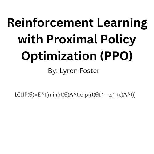
Reinforcement Learning with Proximal Policy Optimization (PPO)

Reinforcement Learning (RL) has been a popular topic in the AI community, especially with its potential in training agents to perform tasks in environments where the correct decision isn’t always obvious. One of the most widely used algorithms in RL is Proximal Policy Optimization (PPO). In this tutorial, we’ll discuss its foundational concepts and implement it from scratch.

Traditional policy gradient methods often face challenges in terms of convergence and stability. PPO was introduced as a more stable and robust alternative. PPO’s key idea is to limit the change in policy at each update, ensuring that the new policy isn’t too different from the old one.

Let’s get up to speed

Before diving in, let’s get familiar with some concepts:

  • Policy: The strategy an agent employs to determine the next action based on the current state.
  • Advantage Function: Indicates how much better an action is compared to the average action at a particular state.
  • Objective Function: For PPO, this function helps in updating the policy in the direction of better performance while ensuring changes aren’t too drastic.

PPO Algorithm

PPO’s Objective Function:

Let’s define:

  • L^CLIP(θ) as the PPO objective we want to maximize.
  • r_t(θ) as the ratio of the probability under the current policy to the probability under the old policy for the action taken at time t.
  • A^_t as the estimated advantage at time t.
  • ε as a small value (typically 0.2) which limits the change in the policy.

The objective function is formulated as:

L^CLIP(θ) = Expected value over time [ min( r_t(θ) * A^_t , clip(r_t(θ), 1-ε, 1+ε) * A^_t ) ]

In simpler terms:

  • Calculate the expected value (or average) over all time steps.
  • For each time step, take the minimum of two values:
  1. The product of the ratio r_t(θ) and the advantage A^_t.
  2. The product of the clipped ratio (restricted between 1-ε and 1+ε) and the advantage A^_t.

The objective ensures that we don’t change the policy too drastically (hence the clipping) while still trying to improve it (using the advantage function).

Implementation

First, let’s define some preliminary code and imports:

import numpy as np
import tensorflow as tf

class PolicyNetwork(tf.keras.Model):
    def __init__(self, n_actions):
        super(PolicyNetwork, self).__init__()
        self.fc1 = tf.keras.layers.Dense(128, activation='relu')
        self.fc2 = tf.keras.layers.Dense(128, activation='relu')
        self.out = tf.keras.layers.Dense(n_actions, activation='softmax')
    
    def call(self, x):
        x = self.fc1(x)
        x = self.fc2(x)
        return self.out(x)

The policy network outputs a probability distribution over actions.

Now, the main PPO update:

def ppo_update(policy, states, actions, advantages, old_probs, epochs=10, clip_epsilon=0.2):
    for _ in range(epochs):
        with tf.GradientTape() as tape:
            probs = policy(states)
            probs = tf.gather(probs, actions, batch_dims=1)
            old_probs = tf.gather(old_probs, actions, batch_dims=1)
            
            r = probs / (old_probs + 1e-10)
            loss = -tf.reduce_mean(tf.minimum(
                r * advantages,
                tf.clip_by_value(r, 1-clip_epsilon, 1+clip_epsilon) * advantages
            ))

grads = tape.gradient(loss, policy.trainable_variables)
        optimizer.apply_gradients(zip(grads, policy.trainable_variables))

To train an agent in a complex environment, you might consider using the OpenAI Gym. Here’s a rough skeleton:

import gym

env = gym.make('Your-Environment-Name-Here')
policy = PolicyNetwork(env.action_space.n)
optimizer = tf.keras.optimizers.Adam(learning_rate=0.001)
for i_episode in range(1000):  # Train for 1000 episodes
    observation = env.reset()
    done = False
    while not done:
        action_probabilities = policy(observation)
        action = np.random.choice(env.action_space.n, p=action_probabilities.numpy())
        
        next_observation, reward, done, _ = env.step(action)
        
        # Calculate advantage, old_probs, etc.
        # ...
        
        ppo_update(policy, states, actions, advantages, old_probs)
        
        observation = next_observation

PPO is an effective algorithm for training agents in various environments. While the above is a simplistic overview, it captures the essence of PPO. For more intricate environments, consider using additional techniques like normalization, entropy regularization, and more sophisticated neural network architectures.

Navigating the Path: Exploring the Pros and Cons of Regulating AI

Navigating the Path: Exploring the Pros and Cons of Regulating AI

Artificial Intelligence (AI) has evolved at an unprecedented pace, permeating various aspects of our lives. From autonomous vehicles to virtual assistants and complex algorithms, AI has become deeply intertwined with our daily routines. However, as this powerful technology continues to advance, questions regarding the need for regulation have emerged. In this article, we will delve into the multifaceted topic of regulating AI, examining both the benefits and challenges that accompany such measures.

The Potential Benefits of Regulating AI

  1. Ethical Framework: One of the primary motivations behind regulating AI is to establish an ethical framework that guides its development and deployment. AI systems possess the ability to make autonomous decisions that have a profound impact on individuals and society as a whole. By implementing regulations, we can ensure that AI is developed and utilized in a manner that aligns with our shared values and ethical principles.
  2. Safety and Security: AI-powered systems can wield immense power, and if left unchecked, they could potentially pose risks to safety and security. Regulating AI can promote the implementation of safeguards and standards that mitigate potential threats. This includes addressing issues such as bias in AI algorithms, ensuring data privacy, and preventing the malicious use of AI technologies.
  3. Transparency and Accountability: AI algorithms can sometimes operate as “black boxes,” making it challenging to comprehend the decision-making processes behind their outputs. By regulating AI, we can encourage transparency and accountability, making it easier to understand how these systems arrive at their conclusions. This fosters trust among users and allows for the identification and rectification of potential biases or errors.

The Challenges of Regulating AI

  1. Innovation and Progress: Overregulation can stifle innovation by burdening AI developers with excessive constraints. Striking the right balance between regulation and fostering innovation is crucial. It is important to avoid impeding the advancement of AI technology, as it holds tremendous potential for addressing complex societal challenges and driving economic growth.
  2. Global Consensus: AI operates on a global scale, and establishing consistent regulations across different countries can be challenging. Varying legal frameworks and cultural differences make it difficult to create unified rules governing AI technology. International collaboration and cooperation will be necessary to address these challenges effectively.
  3. Adaptability and Agility: Technology evolves rapidly, often outpacing the ability to create comprehensive regulations. Prescriptive and rigid regulations may struggle to keep up with the dynamic nature of AI, potentially rendering them obsolete or inadequate. Crafting regulatory frameworks that can adapt to evolving technologies while remaining effective is a complex task.

Balancing Act: A Collaborative Approach

Regulating AI requires a balanced approach that considers the potential benefits and challenges involved. Rather than viewing regulation as a restrictive force, it should be seen as an enabler, fostering responsible and beneficial use of AI technology.

To achieve this, collaboration between various stakeholders is crucial. Governments, industry leaders, AI developers, researchers, and ethicists need to engage in thoughtful dialogue to craft regulations that strike the right balance. This collaborative approach ensures that regulations are informed by technical expertise, societal values, and the concerns of all relevant parties.

Moreover, a continuous feedback loop is necessary to refine regulations as the technology progresses. Regular evaluations, audits, and adaptive frameworks can help ensure that regulations remain effective and up to date.

Regulating AI presents both opportunities and challenges. Establishing a framework that encourages innovation, while safeguarding ethics, safety, and transparency, is key. By engaging in a collaborative approach and embracing continuous learning and adaptation, we can harness the potential of AI while ensuring that it aligns with our shared values. With responsible regulation, we can navigate the path of AI development and deployment, shaping a future where AI serves as a force for positive change.\

What do you think?

What are your thoughts on Regulating AI?

Building an Image Recognition Model Using TensorFlow and Keras in Python

Image recognition, also known as computer vision, is an important field in artificial intelligence. It allows machines to identify and interpret visual information from images, videos, and other visual media. The development of image recognition models has been a game-changer in various industries, such as healthcare, retail, and security. With the advancement of deep learning and neural networks, building an image recognition model has become easier than ever before.

In this article, we will walk you through the process of building an image recognition model using TensorFlow and Keras libraries in Python. TensorFlow is an open-source machine learning library developed by Google that is widely used for building deep learning models. Keras is a high-level neural networks API written in Python that runs on top of TensorFlow, allowing you to build complex neural networks with just a few lines of code.

Before we start, you need to have Python installed on your computer, along with the following libraries – TensorFlow, Keras, NumPy, and Matplotlib. You can install these libraries using pip, a package installer for Python. Once you have installed these libraries, you are ready to start building your image recognition model.

The first step in building an image recognition model is to gather data. You can either collect your own data or use a publicly available dataset. For this example, we will use the CIFAR-10 dataset, which consists of 60,000 32×32 color images in 10 classes, with 6,000 images per class. The classes are – airplane, automobile, bird, cat, deer, dog, frog, horse, ship, and truck.

Once you have the dataset, the next step is to preprocess the data. Preprocessing the data involves converting the images into a format that can be fed into the neural network. In this case, we will convert the images into a matrix of pixel values. We will also normalize the pixel values to be between 0 and 1, which helps the neural network learn faster.

After preprocessing the data, the next step is to build the model. We will use a convolutional neural network (CNN) for this example. A CNN is a type of neural network that is specifically designed for image recognition tasks. It consists of multiple layers, including convolutional layers, pooling layers, and fully connected layers.

The first layer in our CNN is a convolutional layer. The purpose of this layer is to extract features from the input images. We will use 32 filters in this layer, each with a size of 3×3. The activation function we will use is ReLU, which is a commonly used activation function in neural networks.

The next layer is a pooling layer. The purpose of this layer is to downsample the feature maps generated by the convolutional layer. We will use a max pooling layer with a pool size of 2×2.

After the pooling layer, we will add another convolutional layer with 64 filters and a size of 3×3. We will again use the ReLU activation function.

We will then add another max pooling layer with a pool size of 2×2. After the pooling layer, we will add a flattening layer, which converts the 2D feature maps into a 1D vector.

The next layer is a fully connected layer with 128 neurons. We will use the ReLU activation function in this layer as well.

Finally, we will add an output layer with 10 neurons, one for each class in the CIFAR-10 dataset. We will use the softmax activation function in this layer, which is commonly used for multi-class classification tasks.

Once the model is built, we will compile it and train it using the CIFAR-10 dataset. We will use the categorical cross-entropy loss function and the Adam optimizer for training the model. We will also set aside 20% of the data for validation during training.

After training the model, we will evaluate its performance on a test set. We will use the accuracy metric to evaluate the model’s performance. We will also plot the training and validation accuracy and loss curves to visualize the model’s performance during training.

In conclusion, building an image recognition model using TensorFlow and Keras libraries in Python is a straightforward process. With the right dataset and preprocessing techniques, you can build a powerful image recognition model that can accurately classify images into different classes. This technology has a wide range of applications in various industries and is continuously evolving with new advancements in deep learning and neural networks.

Surviving the Rise of A.I. : Evaluating whether or not your job will be replaced by a computer.

Surviving the Rise of A.I. : Evaluating whether or not your job will be replaced by a computer.

As artificial intelligence (AI) continues to advance at a rapid pace, it’s becoming increasingly important for professionals across various industries to understand how this technology might impact their careers. In this article, we will explore the key factors to consider when evaluating whether or not your job can be replaced by AI, as well as offer some insights on how to adapt and thrive in the age of automation.

Understanding AI and Its Capabilities

AI refers to the development of computer systems that can perform tasks that would normally require human intelligence. These tasks include learning, reasoning, problem-solving, perception, and understanding natural language. The capabilities of AI have expanded significantly in recent years due to advancements in machine learning, deep learning, and neural networks.

Job Vulnerability: Routine vs. Non-Routine Tasks

The degree to which a job is susceptible to automation depends largely on the nature of the tasks it involves. In general, jobs that consist mainly of routine tasks are more likely to be replaced by AI. Routine tasks can be divided into two categories:

a. Routine manual tasks: These tasks involve physical labor and are repetitive in nature. Examples include assembly line work, packaging, and sorting.

b. Routine cognitive tasks: These tasks involve mental labor and are also repetitive. Examples include data entry, basic accounting, and scheduling.

Non-routine tasks, on the other hand, are less likely to be replaced by AI. These tasks typically involve problem-solving, critical thinking, creativity, and emotional intelligence. Examples include strategic planning, negotiation, and artistic creation.

AI Adoption in Various Industries

AI has already been adopted in many industries, but the extent of its impact varies considerably. To evaluate the likelihood of your job being replaced by AI, it’s essential to examine the specific industry you work in and assess the current state of AI adoption in that sector. Some of the industries where AI has made significant inroads include:

a. Manufacturing: AI-powered robots have been used to streamline production processes, optimize supply chains, and perform quality control.

b. Healthcare: AI has been utilized for diagnostics, personalized treatment plans, and drug discovery.

c. Finance: AI-powered algorithms are being used for fraud detection, trading, and risk management.

d. Transportation: Autonomous vehicles and drones are being tested and deployed for deliveries and passenger transport.

The Importance of Human Skills in an AI-Driven World

Despite the increasing capabilities of AI, certain human skills will continue to be in high demand. The ability to empathize with others, communicate effectively, and think critically and creatively will set professionals apart in a job market that’s becoming more automated. By focusing on developing these skills, you can improve your chances of remaining relevant and competitive in the workforce.

Assessing the AI Vulnerability of Your Job

To evaluate the likelihood of your job being replaced by AI, consider the following factors:

a. Task composition: Determine the proportion of routine tasks in your job. The higher the percentage of routine tasks, the more likely it is that your job can be automated.

b. Industry trends: Research your industry to understand the current state of AI adoption and its projected impact on your specific job role.

c. Skill set: Reflect on your unique skill set and identify areas where you can develop and improve in order to remain competitive in an AI-driven job market.

Adapting to the Age of Automation

In order to thrive in the age of automation, it’s crucial to be proactive in adapting to the changes brought about by AI. Here are some steps you can take to prepare for the future of work:

a. Lifelong learning: Continuously update your skills and knowledge by pursuing further education, attending workshops, or taking online courses. This will help you stay relevant and competitive in the job market.

b. Embrace technology: Stay informed about the latest technological advancements in your industry and learn how to use new tools and systems that can enhance your productivity and efficiency.

c. Diversify your skills: Develop a diverse skill set that includes both technical and soft skills, such as creativity, critical thinking, and emotional intelligence. This will make you more adaptable to changes in the job market and less likely to be replaced by AI.

d. Networking: Build and maintain a strong professional network, which can help you stay informed about new job opportunities, industry trends, and potential collaborations.

e. Focus on problem-solving: Seek out opportunities to tackle complex challenges and develop innovative solutions. These experiences will help you build a strong portfolio of accomplishments that showcase your ability to thrive in an AI-driven world.

The rise of AI and automation will undoubtedly have a profound impact on the job market in the coming years. By understanding the factors that determine whether your job is at risk of being replaced by AI and taking proactive steps to adapt to the changing landscape, you can ensure that you remain a valuable and competitive member of the workforce.

In conclusion, it’s important to remember that AI technology is not an enemy to be feared, but rather a powerful tool that can be harnessed to improve productivity and create new opportunities. By embracing change and focusing on the development of in-demand human skills, professionals across all industries can adapt and thrive in the age of automation.

Kubeflow Pipelines: A Step-by-Step Guide

Kubeflow Pipelines: A Step-by-Step Guide

Kubeflow Pipelines is a platform for building, deploying, and managing end-to-end machine learning workflows. It streamlines the process of creating and executing ML pipelines, making it easier for data scientists and engineers to collaborate on model development and deployment. In this tutorial, we will guide you through the process of setting up Kubeflow Pipelines on your local machine using MiniKF and running a simple pipeline in Python.

Prerequisites

Step 1: Install Vagrant

First, you need to install Vagrant on your machine. Follow the installation instructions for your operating system here: https://www.vagrantup.com/docs/installation

Step 2: Set up MiniKF

Now, let’s set up MiniKF (Mini Kubeflow) on your local machine. MiniKF is a lightweight version of Kubeflow that runs on top of VirtualBox using Vagrant. It is perfect for testing and development purposes.

Create a new directory for your MiniKF setup and navigate to it in your terminal:

mkdir minikf
cd minikf

Initialize the MiniKF Vagrant box by running:

vagrant init arrikto/minikf

Start the MiniKF virtual machine:

vagrant up

This process will take some time, as Vagrant downloads the MiniKF box and sets up the virtual machine.

Step 3: Access the Kubeflow Dashboard

After the virtual machine is up and running, you can access the Kubeflow dashboard in your browser. Open the following URL: http://10.10.10.10. You will be prompted to log in with a username and password. Use admin as both the username and password.

Step 4: Create a Simple Pipeline in Python

Now, let’s create a simple pipeline in Python that reads some data, processes it, and outputs the result. First, install the Kubeflow Pipelines SDK:

pip install kfp

Create a new Python script (e.g., simple_pipeline.py) and add the following code:

import kfp
from kfp import dsl

def read_data_op():
    return dsl.ContainerOp(
        name="Read Data",
        image="python:3.7",
        command=["sh", "-c"],
        arguments=["echo 'Reading data' && sleep 5"],
    )
def process_data_op():
    return dsl.ContainerOp(
        name="Process Data",
        image="python:3.7",
        command=["sh", "-c"],
        arguments=["echo 'Processing data' && sleep 5"],
    )
def output_data_op():
    return dsl.ContainerOp(
        name="Output Data",
        image="python:3.7",
        command=["sh", "-c"],
        arguments=["echo 'Outputting data' && sleep 5"],
    )
@dsl.pipeline(
    name="Simple Pipeline",
    description="A simple pipeline that reads, processes, and outputs data."
)
def simple_pipeline():
    read_data = read_data_op()
    process_data = process_data_op().after(read_data)
    output_data = output_data_op().after(process_data)
if __name__ == "__main__":
    kfp.compiler.Compiler().compile(simple_pipeline, "simple_pipeline.yaml")

This Python script defines a simple pipeline with three steps: reading data, processing data, and outputting data. Each step is defined as a function that returns a ContainerOp object, which represents a containerized operation in the pipeline. The @dsl.pipeline decorator is used to define the pipeline, and the kfp.compiler.Compiler().compile() function is used to compile the pipeline into a YAML file.

Step 5: Upload and Run the Pipeline

Now that you have created a simple pipeline in Python, let’s upload and run it on the Kubeflow Pipelines platform.

Step 6: Monitor the Pipeline Run

After starting the pipeline run, you will be redirected to the “Run details” page. Here, you can monitor the progress of your pipeline, view the logs for each step, and inspect the output artifacts.

Congratulations! You have successfully set up Kubeflow Pipelines on your local machine, created a simple pipeline in Python, and executed it using the Kubeflow platform. You can now experiment with more complex pipelines, integrate different components, and optimize your machine learning workflows.

With Kubeflow Pipelines, you can automate your machine learning workflows, making it easier to build, deploy, and manage complex ML models. Now that you have a basic understanding of how to create and run pipelines in Kubeflow, you can explore more advanced features and build more sophisticated pipelines for your own projects.

AutoML: Automated Machine Learning in Python

AutoML: Automated Machine Learning in Python

AutoML (Automated Machine Learning) is a branch of machine learning that uses artificial intelligence and machine learning techniques to automate the entire machine learning process. AutoML automates tasks such as data preparation, feature engineering, algorithm selection, hyperparameter tuning, and model evaluation. AutoML enables non-experts to build and deploy machine learning models with minimal effort and technical knowledge.

Automated Machine Learning in Python

Python is a popular language for machine learning, and several libraries support AutoML. In this tutorial, we will use the H2O library to perform AutoML in Python.

Install Library

We will start by installing the H2O library.

pip install h2o

Import Libraries

Next, we will import the necessary libraries, including H2O for AutoML, and NumPy and Pandas for data processing.

import numpy as np
import pandas as pd
import h2o
from h2o.automl import H2OAutoML

Load Data

Next, we will load the data to train the AutoML model

# Load data
url = "https://archive.ics.uci.edu/ml/machine-learning-databases/iris/iris.data"
data = pd.read_csv(url, header=None, names=['sepal_length', 'sepal_width', 'petal_length', 'petal_width', 'class'])

# Convert data to H2O format
h2o.init()
h2o_data = h2o.H2OFrame(data)

In this example, we load the Iris dataset from a URL and convert it to the H2O format.

Train AutoML Model

Next, we will train an AutoML model on the data.

# Train AutoML model
aml = H2OAutoML(max_models=10, seed=1)
aml.train(x=['sepal_length', 'sepal_width', 'petal_length', 'petal_width'], y='class', training_frame=h2o_data)

In this example, we train an AutoML model with a maximum of 10 models and a random seed of 1.

View Model Leaderboard

Next, we can view the leaderboard of the trained models.

# View model leaderboard
lb = aml.leaderboard
print(lb)

In this example, we print the leaderboard of the trained models.

Test AutoML Model

Finally, we can use the trained AutoML model to make predictions on new data.

# Test AutoML model
test_data = pd.DataFrame(np.array([[5.1, 3.5, 1.4, 0.2], [7.7, 3.0, 6.1, 2.3]]), columns=['sepal_length', 'sepal_width', 'petal_length', 'petal_width'])
h2o_test_data = h2o.H2OFrame(test_data)
preds = aml.predict(h2o_test_data)
print(preds)

In this example, we use the trained AutoML model to predict the class of two new data points.

In this tutorial, we covered the basics of AutoML and how to use it in Python to automate the entire machine learning process. AutoML enables non-experts to build and deploy machine learning models with minimal effort and technical knowledge. I hope you found this tutorial useful in understanding AutoML in Python.

Unsupervised Learning: Clustering and Dimensionality Reduction in Python

Unsupervised Learning: Clustering and Dimensionality Reduction in Python

Unsupervised learning is a type of machine learning where the model is not provided with labeled data. The model learns the underlying structure and patterns in the data without any specific guidance on what to look for. Clustering and Dimensionality Reduction are two important techniques in unsupervised learning.

Clustering

Clustering is a technique where the model tries to identify groups in the data based on their similarities. The objective is to group similar data points together and separate dissimilar data points. Clustering algorithms can be used for a variety of applications such as customer segmentation, anomaly detection, and image segmentation.

Dimensionality Reduction

Dimensionality reduction is a technique where the model tries to reduce the number of features in the data while retaining as much information as possible. This is useful when dealing with high-dimensional data where it’s difficult to visualize and analyze the data. Dimensionality reduction algorithms can be used for a variety of applications such as data compression, feature extraction, and visualization.

Clustering Algorithms

There are several clustering algorithms in machine learning, each with its own strengths and weaknesses. In this tutorial, we will cover two popular clustering algorithms: K-Means Clustering and Hierarchical Clustering.

K-Means Clustering

K-Means Clustering is a simple and efficient clustering algorithm. The algorithm partitions the data into K clusters based on their similarity. The number of clusters K is specified by the user. The algorithm starts by randomly selecting K data points as the initial centroids. The data points are then assigned to the nearest centroid based on their distance. The centroid is then updated based on the mean of the data points in the cluster. This process is repeated until convergence.

Let’s see how to implement K-Means Clustering in Python using Scikit-Learn.

from sklearn.cluster import KMeans
import numpy as np

# Generate random data
X = np.random.rand(100, 2)
# Initialize KMeans model with 2 clusters
kmeans = KMeans(n_clusters=2)
# Fit the model to the data
kmeans.fit(X)
# Predict the clusters for the data
y_pred = kmeans.predict(X)
# Print the centroids of the clusters
print(kmeans.cluster_centers_)

In this example, we generate random data with 2 features and 100 data points. We then initialize the KMeans model with 2 clusters and fit the model to the data. We then predict the clusters for the data and print the centroids of the clusters.

Hierarchical Clustering

Hierarchical Clustering is a clustering algorithm that builds a hierarchy of clusters. The algorithm starts by treating each data point as a separate cluster. The algorithm then iteratively merges the closest clusters based on their distance until all the data points belong to a single cluster.

There are two types of hierarchical clustering algorithms: Agglomerative and Divisive. Agglomerative clustering starts with each data point as a separate cluster and iteratively merges the closest clusters. Divisive clustering starts with all data points in a single cluster and iteratively splits the cluster into smaller clusters.

Let’s see how to implement Agglomerative Hierarchical Clustering in Python using Scikit-Learn.

from sklearn.cluster import AgglomerativeClustering
import numpy as np

# Generate random data
X = np.random.rand(100, 2)
# Initialize AgglomerativeClustering model with 2 clusters
agg_clustering = AgglomerativeClustering(n_clusters=2)
# Fit the model to the data
agg_clustering.fit(X)
# Predict the clusters for the data
y_pred = agg_clustering.labels_
# Print the labels of the clusters
print(y_pred)

In this example, we generate random data with 2 features and 100 data points. We then initialize the AgglomerativeClustering model with 2 clusters and fit the model to the data. We then predict the clusters for the data and print the labels of the clusters.

Divisive Hierarchical Clustering

Divisive Hierarchical Clustering is a clustering algorithm that starts with all data points in a single cluster and iteratively splits the cluster into smaller clusters. The algorithm starts by treating all data points as a single cluster. The algorithm then iteratively splits the cluster into smaller clusters based on their dissimilarity until each data point belongs to a separate cluster.

Divisive Hierarchical Clustering is not as popular as Agglomerative Hierarchical Clustering because it is computationally expensive and tends to produce imbalanced clusters.

Dimensionality Reduction Algorithms

There are several dimensionality reduction algorithms in machine learning, each with its own strengths and weaknesses. In this tutorial, we will cover two popular dimensionality reduction algorithms: Principal Component Analysis (PCA) and t-Distributed Stochastic Neighbor Embedding (t-SNE).

Principal Component Analysis (PCA)

Principal Component Analysis (PCA) is a linear dimensionality reduction technique that tries to find the orthogonal directions of maximum variance in the data. The objective is to find a lower-dimensional representation of the data that retains as much information as possible. PCA is useful when dealing with high-dimensional data where it’s difficult to visualize and analyze the data.

Let’s see how to implement PCA in Python using Scikit-Learn.

from sklearn.decomposition import PCA
import numpy as np

# Generate random data
X = np.random.rand(100, 10)
# Initialize PCA model with 2 components
pca = PCA(n_components=2)
# Fit the model to the data
pca.fit(X)
# Transform the data to 2 dimensions
X_transformed = pca.transform(X)
# Print the shape of the transformed data
print(X_transformed.shape)

In this example, we generate random data with 10 features and 100 data points. We then initialize the PCA model with 2 components and fit the model to the data. We then transform the data to 2 dimensions and print the shape of the transformed data.

t-Distributed Stochastic Neighbor Embedding (t-SNE)

t-Distributed Stochastic Neighbor Embedding (t-SNE) is a nonlinear dimensionality reduction technique that tries to preserve the pairwise distances between the data points in the lower-dimensional representation. The objective is to find a lower-dimensional representation of the data that retains the local structure of the data. t-SNE is useful when dealing with high-dimensional data where it’s difficult to visualize and analyze the data.

Let’s see how to implement t-SNE in Python using Scikit-Learn.

from sklearn.manifold import TSNE
import numpy as np

# Generate random data
X = np.random.rand(100, 10)
# Initialize t-SNE model with 2 components
tsne = TSNE(n_components=2)
# Fit the model to the data
X_transformed = tsne.fit_transform(X)
# Print the shape of the transformed data
print(X_transformed.shape)

In this example, we generate random data with 10 features and 100 data points. We then initialize the t-SNE model with 2 components and fit the model to the data. We then transform the data to 2 dimensions and print the shape of the transformed data.

In this tutorial, we covered two important techniques in unsupervised learning: Clustering and Dimensionality Reduction. We also covered two popular algorithms for each technique: K-Means Clustering and Hierarchical Clustering for Clustering, and PCA and t-SNE for Dimensionality Reduction. We also provided code examples in Python using Scikit-Learn.

I hope you found this tutorial useful in understanding Unsupervised Learning. To learn more about Machine Learning, I hope you will consider checking out my book: Unsupervised Learning: Clustering and Dimensionality Reduction (https://a.co/d/3AQdFnG)

Fraud Detection with Machine Learning using Python (numpy, pandas, matplotlib, and scikit-learn)

Fraud Detection with Machine Learning using Python (numpy, pandas, matplotlib, and scikit-learn)

Fraud is a pervasive problem in many industries, including finance, insurance, and social media. With the increasing availability of data and the advancement of machine learning algorithms, it has become possible to leverage these tools to detect fraudulent activity more effectively.

In this post, I’ll explore how machine learning can be used for fraud detection. I’ll going to create a tutorial demonstrating how to implement a fraud detection model using Python.

I’ll discuss the key concepts and techniques involved in fraud detection with machine learning, such as preprocessing the data, selecting an appropriate machine learning algorithm, and evaluating the performance of the model.

Sounds cool, right? Let’s dive in!

Step 1. Import the required libraries:

First, you need to import the required libraries, including numpy, pandas, matplotlib, and scikit-learn.

Step 2. Load the data:

Next, you need to load the data that you will use for fraud detection. You can use a publicly available dataset such as the Credit Card Fraud Detection dataset from Kaggle.

Step 3. Explore the data:

Once the data is loaded, you need to explore it to gain a better understanding of its features and distributions.

Step 4. Preprocess the data:

Once you have explored the data, you need to preprocess it so that it can be used for training the machine learning model. This involves tasks such as feature engineering, normalization, and splitting the data into training and validation sets.

In this preprocessing example, we first remove the  column from the dataset as it is not useful for classification. We then normalize the  column using , which scales the data to have a mean of 0 and a standard deviation of 1. This is an important preprocessing step as it ensures that all the features have similar scales, which can help improve the performance of the machine learning model.

Next, we split the data into features () and labels (). The  dataframe contains all the columns except the  column, which is the target variable we are trying to predict. The  dataframe contains only the  column.

Finally, we split the data into training and validation sets using  from scikit-learn. We use a test size of 0.2, which means that 20% of the data is used for validation. We also use stratified sampling to ensure that the proportion of fraudulent and non-fraudulent transactions is the same in both the training and validation sets. This is important as it ensures that the machine learning model is trained on a representative sample of the data.

Step 5. Define the model:

Once the data is preprocessed, you need to define the architecture of the machine learning model. For this example, we will use a random forest classifier.

Step 6. Train the model:

Once the model is defined, you need to train it using the preprocessed data.

Step 7. Evaluate the model:

After training the model, you need to evaluate its performance on the validation set.

Step 8. Test the model:

Once you are satisfied with the model’s performance on the validation set, you can test it on a new set of data to see how well it generalizes to unseen data.

In this testing example, we first load the new data from a CSV file using . We then preprocess the new data by dropping the  column and normalizing the  column using the same  object that we used for the training data.

Next, we split the new data into features () and labels (). We then use the  method to make predictions on the new data. Finally, we evaluate the performance of the model on the new data using  from scikit-learn. This method prints a report that includes metrics such as precision, recall, and F1-score for both the fraudulent and non-fraudulent classes.

This allows us to get a better sense of how well it generalizes to unseen data and how effective it is at detecting fraudulent activity in real-world scenarios.

That’s it! This basic basic example should give you an idea of how to use machine learning for fraud detection using Python.