Concurrency and Goroutines: Understanding Concurrency and Goroutines in Go

May 15, 2023 synchronization

Concurrency and Goroutines: Understanding Concurrency and Goroutines in Go

Concurrency is an essential concept in modern programming, allowing multiple tasks to run concurrently and efficiently utilize system resources. Go, a statically typed programming language developed by Google, provides built-in support for concurrency through Goroutines and channels. In this tutorial, we will explore how to leverage Goroutines and manage concurrency using GoLand, a popular integrated development environment (IDE) for Go.

1. Introduction to Concurrency in Go

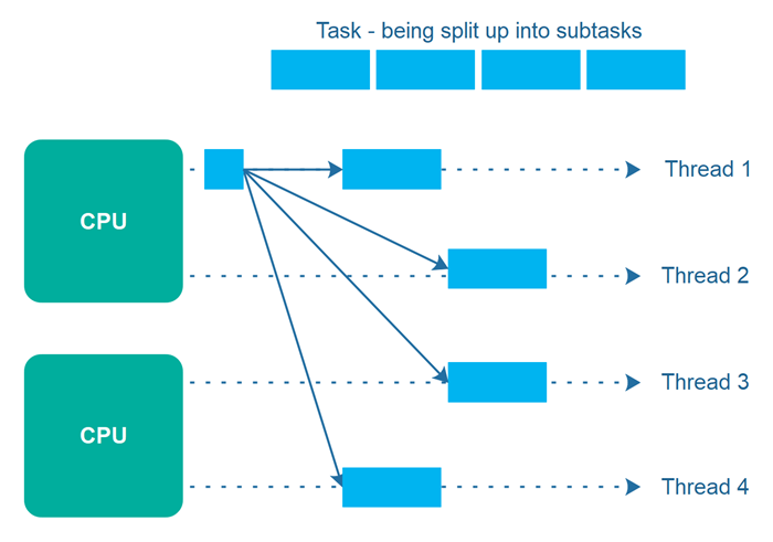
Concurrency is the ability of a program to perform multiple tasks simultaneously, making efficient use of system resources such as CPU cores. Go introduces concurrency as a core language feature, enabling developers to write concurrent programs easily and efficiently.

Go achieves concurrency through Goroutines, which are lightweight concurrent execution units, and channels, which provide synchronization and communication between Goroutines.

2. Goroutines: Lightweight Concurrent Execution Units

A Goroutine is a function that can be executed concurrently with other Goroutines. They are lightweight and have a smaller memory footprint compared to operating system threads. Goroutines are managed by the Go runtime, allowing efficient scheduling and execution of concurrent tasks.

The go keyword is used to start a new Goroutine. When a Goroutine is created, it runs concurrently with the main Goroutine or other Goroutines, allowing parallel execution.

3. Creating and Running Goroutines

Let’s dive into some code examples to see how Goroutines are created and run in Go. Assume we have a function process() that performs some time-consuming task.

func process() {
    // Perform some time-consuming task
}

To execute this function concurrently using a Goroutine, we can use the go keyword:

go process()

The go keyword launches a new Goroutine, and process() will start executing concurrently. The main Goroutine and the newly created Goroutine will run independently.

4. Synchronization with Channels

Channels in Go provide a mechanism for Goroutines to communicate and synchronize their execution. A channel is a typed conduit that allows sending and receiving values between Goroutines.

Let’s consider an example where we have two Goroutines: a producer and a consumer. The producer generates some data and sends it to the consumer using a channel.

func producer(ch chan<- int) {
    for i := 0; i < 5; i++ {
        ch <- i // Send data to the channel
    }
    close(ch) // Close the channel to signal the end of data
}

func consumer(ch <-chan int) {
    for num := range ch {
        fmt.Println(num) // Print the received data
    }
}

In this example, the producer Goroutine sends integers to the channel ch, and the consumer Goroutine receives and prints them. The ch channel is created with the type chan int, indicating it can only send or receive integers.

To execute the producer and consumer concurrently, we can create a channel and launch the Goroutines using the go keyword:

ch := make(chan int)
go producer(ch)
go consumer(ch)

The producer Goroutine sends data to the channel, and the consumer Goroutine receives and prints it. This synchronization ensures that the consumer only processes data when it is available.

5. GoLand’s Tools for Managing Goroutines

GoLand, an IDE developed by JetBrains, provides powerful tools to manage Goroutines and visualize concurrent execution.

Debugging Goroutines

GoLand offers a rich set of debugging features for Goroutines. You can set breakpoints, inspect variables, and step through Goroutines to identify and fix issues in concurrent code.

To debug Goroutines in GoLand, follow these steps:

Set a breakpoint in the code where you want to start debugging.
Run the program in debug mode by clicking on the “Debug” button or using the corresponding keyboard shortcut.
When the breakpoint is hit, the program execution will pause.
Use the debugging toolbar to step through the code, inspect variables, and analyze Goroutine behavior.

Goroutine Visualization

Understanding the flow of Goroutines and how they interact can be challenging in complex concurrent programs. GoLand provides a visual Goroutine tool that helps you analyze the Goroutine execution flow.

To visualize Goroutines in GoLand, follow these steps:

Run your program in debug mode.
Open the “Goroutines” tab in the Debug tool window.
The “Goroutines” tab displays a list of active Goroutines and their current state.
You can see the Goroutine stack traces, examine their state, and navigate through them to understand the execution flow.

Profiling Goroutines

Profiling is crucial for optimizing performance in concurrent programs. GoLand integrates with Go’s profiling tools to help you analyze Goroutine behavior and identify bottlenecks.

To profile Goroutines in GoLand, follow these steps:

Open the “Run” menu and select “Profile”.
Choose the profiling type you want, such as CPU profiling or memory profiling.
Run your program with the selected profiling configuration.
GoLand will collect profiling data and present it in an interactive UI.
Analyze the Goroutine-specific profiling results to identify performance issues and optimize your code.

Concurrency and Goroutines are fundamental to writing efficient and scalable programs in Go. With GoLand’s powerful tools for managing Goroutines, you can debug, visualize, and profile concurrent code effectively.

In this tutorial, we covered the basics of concurrency and Goroutines in Go, including creating and running Goroutines, synchronizing with channels, and leveraging GoLand’s tools for managing Goroutines. Armed with this knowledge, you can confidently write concurrent programs in Go and utilize GoLand’s features to enhance your development workflow.

Remember, concurrency can be complex, so it’s important to understand the principles and best practices to write correct and efficient concurrent code. Keep exploring the vast possibilities of Goroutines and Go’s concurrency features to build robust and highly performant applications.

Demand Clustering and Segmentation with Machine Learning in Logistics (Kmeans, scikit-learn, matplotlib)

May 15, 2023 supply chain optimization

Demand Clustering and Segmentation with Machine Learning in Logistics (Kmeans, scikit-learn, matplotlib)

In the field of logistics, understanding and predicting customer demand patterns is crucial for optimizing supply chain operations. By employing machine learning techniques, we can cluster and segment demand data to uncover valuable insights and make informed decisions. In this tutorial, we will explore how to perform demand clustering and segmentation using Python and popular machine learning libraries.

Prereqs

To follow along with this tutorial, you’ll need:

Python 3.x installed on your system
The following Python libraries: pandas, numpy, scikit-learn, matplotlib

You can install the required libraries using pip:

pip install pandas numpy scikit-learn matplotlib

Step 1: Data Preparation

The first step is to gather and prepare the demand data for analysis. This typically involves loading the data into a pandas DataFrame and performing any necessary preprocessing steps such as handling missing values or normalizing the data. For this tutorial, we’ll assume you have a CSV file containing demand data with the following columns: date, product_id, quantity.

Let’s start by importing the necessary libraries and loading the data:

import pandas as pd

# Load the demand data from CSV
demand_data = pd.read_csv('demand_data.csv')

Next, we can examine the data and perform any necessary preprocessing steps. This might include handling missing values, converting data types, or normalizing the data. Preprocessing steps will vary depending on the specific dataset and requirements of your analysis.

Step 2: Feature Engineering

To apply machine learning algorithms, we need to extract relevant features from the demand data. In this tutorial, we’ll use the following features: product_id, quantity, and date (as a temporal feature). We’ll transform the date column into separate features such as year, month, day, and day of the week. Additionally, we can include other domain-specific features if available, such as product category or customer segment.

Let’s create a function to perform feature engineering:

from datetime import datetime

def engineer_features(data):
    # Convert date column to datetime
    data['date'] = pd.to_datetime(data['date'])
    # Extract year, month, day, and day of the week
    data['year'] = data['date'].dt.year
    data['month'] = data['date'].dt.month
    data['day'] = data['date'].dt.day
    data['day_of_week'] = data['date'].dt.dayofweek
    # Include other relevant features if available
    return data
# Apply feature engineering
demand_data = engineer_features(demand_data)

Step 3: Demand Clustering

Now that we have prepared our data and engineered the necessary features, we can proceed with demand clustering. Clustering is an unsupervised learning technique that groups similar instances together based on their features. In our case, we want to cluster demand patterns based on the extracted features.

For this tutorial, we’ll use the popular K-means clustering algorithm. Let’s import the required libraries and perform the clustering:

from sklearn.cluster import KMeans

# Select relevant features for clustering
features = ['quantity', 'year', 'month', 'day', 'day_of_week']
# Perform clustering
kmeans = KMeans(n_clusters=3)
clusters = kmeans.fit_predict(demand_data[features])

In the code above, we selected the features to be used for clustering (quantity, year, month, day, day_of_week) and specified the number of clusters to be 3. You can adjust these parameters according to your specific use case.

Step 4: Demand Segmentation

Once we have performed demand clustering, we can further segment the clusters to gain deeper insights into different customer demand patterns. Segmentation helps us understand distinct groups within each cluster, allowing us to tailor our logistics strategies accordingly.

In this tutorial, we’ll use the K-means clustering results to perform segmentation. We’ll calculate the centroid of each cluster and assign demand data points to the nearest centroid. This will help us identify which products or time periods belong to each segment within a cluster.

Let’s continue with the code:

# Add cluster labels to the demand data
demand_data['cluster'] = clusters

# Calculate the centroid of each cluster
cluster_centroids = pd.DataFrame(kmeans.cluster_centers_, columns=features)
# Segment the demand data based on cluster centroids
segment_labels = kmeans.predict(cluster_centroids)
demand_data['segment'] = demand_data['cluster'].apply(lambda x: segment_labels[x])

In the code above, we added the cluster labels to the demand data. Then, we calculated the centroid of each cluster using the cluster_centers_ attribute of the K-means model. Next, we predicted the segment labels for each cluster centroid using the predict method. Finally, we assigned the segment labels to the demand data based on their corresponding cluster.

Step 5: Visualizing Clusters and Segments

To better understand the clustering and segmentation results, it’s helpful to visualize them. We can plot the clusters and segments on different charts to observe patterns and identify differences between them.

Let’s create a scatter plot to visualize the clusters:

import matplotlib.pyplot as plt

# Plot clusters
plt.scatter(demand_data['quantity'], demand_data['year'], c=demand_data['cluster'])
plt.xlabel('Quantity')
plt.ylabel('Year')
plt.title('Demand Clusters')
plt.show()

Similarly, we can create a bar chart to visualize the segments:

segment_counts = demand_data['segment'].value_counts()

# Plot segments
plt.bar(segment_counts.index, segment_counts.values)
plt.xlabel('Segment')
plt.ylabel('Count')
plt.title('Demand Segments')
plt.show()

By visualizing the clusters and segments, we can gain insights into the distinct demand patterns within our data. This information can be used to make data-driven decisions and optimize logistics operations accordingly.

In this tutorial, we explored how to perform demand clustering and segmentation using machine learning in logistics. We learned how to prepare the data, engineer relevant features, apply clustering algorithms, and segment the results. Additionally, we visualized the clusters and segments to gain insights into the demand patterns.

By employing these techniques, logistics professionals can effectively analyze customer demand, uncover hidden patterns, and optimize their supply chain operations for improved efficiency and customer satisfaction.

Remember, demand clustering and segmentation is just one aspect of utilizing machine learning in logistics. There are many other techniques and models that can be applied to tackle different challenges in the field. So feel free to explore further and expand your knowledge!

Happy coding!

Predicting Delivery Time and Estimating Shipment Delays with Machine Learning (Supply Chain and Logistics Series)

May 14, 2023 logistics

Predicting Delivery Time and Estimating Shipment Delays with Machine Learning (Supply Chain and Logistics Series)

In today’s fast-paced world, efficient delivery and logistics are crucial for businesses. Predicting delivery times accurately and estimating shipment delays can help companies streamline their operations, optimize resources, and provide better customer service. Machine learning techniques can be employed to analyze historical data and build predictive models that can forecast delivery times and identify potential delays. In this tutorial, we will explore how to use Python and machine learning to predict delivery time and estimate shipment delays.

1. Understanding the Problem

Before diving into the implementation, let’s understand the problem we are trying to solve. Our goal is to predict the delivery time for shipments and estimate potential delays based on historical data. We will use machine learning algorithms to train a model that can learn from past deliveries and make predictions on new, unseen data.

2. Gathering and Preparing the Data

To build our predictive model, we need a dataset that includes information about past deliveries, such as shipment details, timestamps, and actual delivery times. This data can be obtained from various sources, including internal company records or publicly available datasets.

Once we have collected the data, we need to preprocess and prepare it for the machine learning model. This involves tasks such as handling missing values, encoding categorical variables, and scaling numerical features. Python libraries such as Pandas and Scikit-learn are excellent tools for data preprocessing.

import pandas as pd
from sklearn.model_selection import train_test_split

# Load the dataset
data = pd.read_csv('delivery_data.csv')
# Separate the features and target variable
X = data.drop('delivery_time', axis=1)
y = data['delivery_time']
# Split the data into training and testing sets
X_train, X_test, y_train, y_test = train_test_split(X, y, test_size=0.2, random_state=42)

3. Exploratory Data Analysis (EDA)

EDA is a crucial step in any data analysis project. It helps us understand the structure and patterns present in the data. During EDA, we can perform tasks such as visualizing the distribution of features, identifying outliers, and examining relationships between variables. Matplotlib and Seaborn are popular Python libraries for data visualization.

import matplotlib.pyplot as plt
import seaborn as sns

# Visualize the distribution of the target variable
sns.histplot(data['delivery_time'], kde=True)
plt.xlabel('Delivery Time')
plt.ylabel('Count')
plt.title('Distribution of Delivery Time')
plt.show()
# Explore the relationship between features and the target variable
sns.scatterplot(data['distance'], data['delivery_time'])
plt.xlabel('Distance')
plt.ylabel('Delivery Time')
plt.title('Delivery Time vs Distance')
plt.show()

4. Feature Engineering

Feature engineering involves creating new features or transforming existing ones to enhance the predictive power of our model. In the context of delivery time prediction, we can extract useful information from the existing features, such as the day of the week, hour of the day, or distance between the origin and destination. Feature engineering requires domain knowledge and creativity to capture relevant information that can improve the model’s performance.

# Extract day of the week and hour of the day from timestamps
X['day_of_week'] = pd.to_datetime(X['timestamp']).dt.dayofweek
X['hour_of_day'] = pd.to_datetime(X['timestamp']).dt.hour

# Calculate the distance between origin and destination
X['distance'] = ((X['destination_x'] - X['origin_x'])**2 + (X['destination_y'] - X['origin_y'])**2)**0.5

5. Splitting the Data

Before building our machine learning model, we need to split the dataset into training and testing sets. The training set will be used to train the model, while the testing set will be used to evaluate its performance on unseen data. The Scikit-learn library provides convenient functions to split the data into training and testing sets.

from sklearn.model_selection import train_test_split

# Split the data into training and testing sets
X_train, X_test, y_train, y_test = train_test_split(X, y, test_size=0.2, random_state=42)

6. Building the Machine Learning Model

Now it’s time to build our machine learning model. There are several algorithms we can use for regression tasks, including linear regression, decision trees, random forests, or gradient boosting. Each algorithm has its strengths and weaknesses, and the choice depends on the specific problem and dataset. Scikit-learn provides implementations of various regression algorithms that we can use to build our model.

from sklearn.linear_model import LinearRegression

# Initialize the linear regression model
model = LinearRegression()

# Train the model
model.fit(X_train, y_train)

7. Model Evaluation

After training our model, we need to evaluate its performance to ensure its effectiveness. Common evaluation metrics for regression tasks include mean absolute error (MAE), mean squared error (MSE), and R-squared. We can use these metrics to assess how well our model predicts the delivery time and estimate the potential delays.

from sklearn.metrics import mean_absolute_error, mean_squared_error, r2_score

# Make predictions on the test set
y_pred = model.predict(X_test)

# Calculate evaluation metrics
mae = mean_absolute_error(y_test, y_pred)
mse = mean_squared_error(y_test, y_pred)
r2 = r2_score(y_test, y_pred)

print("Mean Absolute Error (MAE):", mae)
print("Mean Squared Error (MSE):", mse)
print("R-squared Score (R2):", r2)

8. Predicting Delivery Time and Estimating Shipment Delays

Once we have built and evaluated our model, we can use it to make predictions on new, unseen data. Given a set of features for a shipment, our model can predict the delivery time and estimate potential delays.

# Create a new shipment with features
new_shipment = pd.DataFrame({'timestamp': ['2023-05-15 10:30:00'],
                             'origin_x': [40.7128],
                             'origin_y': [-74.0060],
                             'destination_x': [34.0522],
                             'destination_y': [-118.2437],
                             'distance': [0],
                             'day_of_week': [0],
                             'hour_of_day': [10]})

# Make a prediction on the new shipment
predicted_delivery_time = model.predict(new_shipment)

print("Predicted Delivery Time:", predicted_delivery_time)

By following this tutorial, you have learned how to predict delivery time and estimate shipment delays using machine learning techniques in Python. This can greatly assist businesses in optimizing their operations and providing better customer service. Remember to continuously iterate and improve your model by experimenting with different algorithms, feature engineering techniques, and evaluation metrics.

In conclusion, predicting delivery time and estimating shipment delays with machine learning can be a valuable tool for businesses in the logistics industry. It allows them to make data-driven decisions, optimize their operations, and provide better service to their customers. By following the steps outlined in this tutorial and leveraging the power of Python and machine learning libraries, you can build accurate prediction models that will contribute to the success of your delivery operations.

Happy coding!

Deep Learning for Medical Genomics and Genetics with Python and TensorFlow

May 13, 2023 artificial intelligence deep learning Machine Learning tensorflow

Deep Learning for Medical Genomics and Genetics with Python and TensorFlow

Deep learning has emerged as a powerful tool in the field of medical genomics and genetics, enabling researchers and healthcare professionals to analyze and interpret large-scale genomic data. In this tutorial, we will explore how to apply deep learning techniques using Python and TensorFlow, a popular deep learning framework, to address various challenges in medical genomics and genetics.

Prereqs

To follow along with this tutorial, you should have a basic understanding of genomics and genetics concepts, as well as some knowledge of Python programming and deep learning principles. You will also need to have TensorFlow installed on your system. If you haven’t installed it yet, you can use the following command to install it using pip:

pip install tensorflow

1. Data Preparation

Before diving into deep learning models, we need to prepare our genomic data for training. This step usually involves preprocessing, cleaning, and transforming the raw genomic data into a format suitable for deep learning models. Let’s assume we have a dataset consisting of genomic sequences and corresponding labels indicating the presence or absence of a certain genetic variant.

# Import necessary libraries
import numpy as np

# Load the genomic data
data = np.load('genomic_data.npy')
labels = np.load('genomic_labels.npy')
# Split the dataset into training and testing sets
train_data = data[:800]
train_labels = labels[:800]
test_data = data[800:]
test_labels = labels[800:]

2. Building a Convolutional Neural Network (CNN)

Convolutional Neural Networks (CNNs) are widely used in genomics for their ability to capture local patterns and dependencies in genomic sequences. Let’s create a simple CNN model using TensorFlow for our genomic classification task.

from tensorflow.keras.models import Sequential
from tensorflow.keras.layers import Conv1D, MaxPooling1D, Flatten, Dense

# Create a CNN model
model = Sequential()
model.add(Conv1D(filters=32, kernel_size=3, activation='relu', input_shape=(100, 4)))
model.add(MaxPooling1D(pool_size=2))
model.add(Flatten())
model.add(Dense(64, activation='relu'))
model.add(Dense(1, activation='sigmoid'))
# Compile the model
model.compile(optimizer='adam', loss='binary_crossentropy', metrics=['accuracy'])
# Train the model
model.fit(train_data, train_labels, epochs=10, batch_size=32)
# Evaluate the model on the test set
loss, accuracy = model.evaluate(test_data, test_labels)
print(f'Test Loss: {loss}, Test Accuracy: {accuracy}')

3. Recurrent Neural Networks (RNN) for Sequence Analysis

Recurrent Neural Networks (RNNs) are particularly useful for modeling sequential data such as genomic sequences. Let’s build an RNN model using LSTM (Long Short-Term Memory) units.

from tensorflow.keras.layers import LSTM

# Create an RNN model
model = Sequential()
model.add(LSTM(units=64, input_shape=(100, 4)))
model.add(Dense(1, activation='sigmoid'))
# Compile the model
model.compile(optimizer='adam', loss='binary_crossentropy', metrics=['accuracy'])
# Train the model
model.fit(train_data, train_labels, epochs=10, batch_size=32)
# Evaluate the model on the test set
loss, accuracy = model.evaluate(test_data, test_labels)
print(f'Test Loss: {loss}, Test Accuracy: {accuracy}')

4. Transfer Learning with Pretrained Models

Transfer learning allows us to leverage preexisting knowledge from large-scale genomics datasets to improve the performance of our models in medical genomics and genetics. We can utilize pretrained models, such as those trained on large genomics datasets like the Genomic Data Commons (GDC) or The Cancer Genome Atlas (TCGA). Here’s an example of how to perform transfer learning using a pretrained model:

from tensorflow.keras.applications import VGG16

# Load the pretrained VGG16 model
base_model = VGG16(weights='imagenet', include_top=False, input_shape=(100, 100, 3))
# Freeze the base model layers
for layer in base_model.layers:
    layer.trainable = False
# Create a new model on top of the pretrained base model
model = Sequential()
model.add(base_model)
model.add(Flatten())
model.add(Dense(64, activation='relu'))
model.add(Dense(1, activation='sigmoid'))
# Compile the model
model.compile(optimizer='adam', loss='binary_crossentropy', metrics=['accuracy'])
# Train the model
model.fit(train_data, train_labels, epochs=10, batch_size=32)
# Evaluate the model on the test set
loss, accuracy = model.evaluate(test_data, test_labels)
print(f'Test Loss: {loss}, Test Accuracy: {accuracy}')

In this tutorial, we have explored the application of deep learning in the field of medical genomics and genetics using Python and TensorFlow. We covered data preparation, building convolutional and recurrent neural network models, as well as transfer learning with pretrained models. With the knowledge gained from this tutorial, you can start exploring and implementing deep learning techniques to analyze and interpret genomic data for various medical applications.

Remember to keep in mind the unique characteristics and challenges of genomics data, such as sequence length, dimensionality, and class imbalance, when designing and training deep learning models. Experimentation and fine-tuning are essential to achieve optimal performance for your specific genomics tasks.

Happy coding and exploring the exciting intersection of deep learning and medical genomics!

Scaling Machine Learning: Building a Multi-Tenant Learning Model System in Python

May 12, 2023 artificial intelligence Machine Learning Python

Scaling Machine Learning: Building a Multi-Tenant Learning Model System in Python

In the world of machine learning, the ability to handle multiple tenants or clients with their own learning models is becoming increasingly important. Whether you are building a platform for personalized recommendations, predictive analytics, or any other data-driven application, a multi-tenant learning model system can provide scalability, flexibility, and efficiency.

In this tutorial, I will guide you through the process of creating a multi-tenant learning model system using Python. You will learn how to set up the project structure, define tenant configurations, implement learning models, and build a robust system that can handle multiple clients with unique machine learning requirements.

By the end of this tutorial, you will have a solid understanding of the key components involved in building a multi-tenant learning model system and be ready to adapt it to your own projects. So let’s dive in and explore the fascinating world of multi-tenant machine learning!

Step 1: Setting Up the Project Structure

Create a new directory for your project and navigate into it. Then, create the following subdirectories using the terminal or command prompt:

mkdir multi_tenant_learning
cd multi_tenant_learning
mkdir models tenants utils

Step 2: Creating the Tenant Configuration

Create JSON files for each tenant inside the tenants directory. Here, we’ll create two tenant configurations: tenant1.json and tenant2.json. Open your favorite text editor and create tenant1.json with the following contents:

{
  "name": "Tenant 1",
  "model_type": "Linear Regression",
  "hyperparameters": {
    "alpha": 0.01,
    "max_iter": 1000
  }
}

Similarly, create tenant2.json with the following contents:

{
  "name": "Tenant 2",
  "model_type": "Random Forest",
  "hyperparameters": {
    "n_estimators": 100,
    "max_depth": 5
  }
}

Step 3: Defining the Learning Models

Create Python modules for each learning model inside the models directory. Here, we’ll create two model files: model1.py and model2.py. Open your text editor and create model1.py with the following contents:

from sklearn.linear_model import LinearRegression

class Model1:
    def __init__(self, alpha, max_iter):
        self.model = LinearRegression(alpha=alpha, max_iter=max_iter)
    def train(self, X, y):
        self.model.fit(X, y)
    def predict(self, X):
        return self.model.predict(X)

Similarly, create model2.py with the following contents:

from sklearn.ensemble import RandomForestRegressor

class Model2:
    def __init__(self, n_estimators, max_depth):
        self.model = RandomForestRegressor(n_estimators=n_estimators, max_depth=max_depth)
    def train(self, X, y):
        self.model.fit(X, y)
    def predict(self, X):
        return self.model.predict(X)

Step 4: Implementing the Multi-Tenant System

Create main.py in the project directory and open it in your text editor. Add the following code:

import json
import os
from models.model1 import Model1
from models.model2 import Model2

def load_tenant_configurations():
    configs = {}
    tenant_files = os.listdir('tenants')
    for file in tenant_files:
        with open(os.path.join('tenants', file), 'r') as f:
            config = json.load(f)
            configs[file] = config
    return configs
def initialize_models(configs):
    models = {}
    for tenant, config in configs.items():
        if config['model_type'] == 'Linear Regression':
            model = Model1(config['hyperparameters']['alpha'], config['hyperparameters']['max_iter'])
        elif config['model_type'] == 'Random Forest':
            model = Model2(config['hyperparameters']['n_estimators'], config['hyperparameters']['max_depth'])
        else:
            raise ValueError(f"Invalid model type for {config['name']}")
        models[tenant] = model
    return models
def train_models(models, X, y):
    for tenant, model in models.items():
        print(f"Training model for {tenant}")
        model.train(X, y)
        print(f"Training completed for {tenant}\n")

def evaluate_models(models, X_test, y_test):
    for tenant, model in models.items():
        print(f"Evaluating model for {tenant}")
        predictions = model.predict(X_test)
        # Implement your own evaluation metrics here
        # For example:
        # accuracy = calculate_accuracy(predictions, y_test)
        # print(f"Accuracy for {tenant}: {accuracy}\n")
def main():
    configs = load_tenant_configurations()
    models = initialize_models(configs)
    # Load and preprocess your data
    X = ...
    y = ...
    X_test = ...
    y_test = ...
    train_models(models, X, y)
    evaluate_models(models, X_test, y_test)
if __name__ == '__main__':
    main()

In the load_tenant_configurations function, we load the JSON files from the tenants directory and parse the configuration details for each tenant.

The initialize_models function creates instances of the learning models based on the configuration details. It checks the model_type in the configuration and initializes the corresponding model class.

The train_models function trains the models for each tenant using the provided data. You can replace the print statements with actual training code specific to your models and data.

The evaluate_models function evaluates the models using test data. You can implement your own evaluation metrics based on your specific problem and requirements.

Finally, in the main function, we load the configurations, initialize the models, and provide placeholder code for loading and preprocessing your data. You need to replace the placeholders with your actual data loading and preprocessing logic.

To run the multi-tenant learning model system, execute python main.py in the terminal or command prompt.

Remember to install any required libraries (e.g., scikit-learn) using pip before running the code.

That’s it! You’ve created a multi-tenant learning model system in Python. Feel free to customize and extend the code according to your needs. Happy coding!

Big Data on Kubernetes: Streamline Your Big Data Workflows with Ease (Hadoop)

May 10, 2023 Docker.

Kubernetes provides a powerful platform for deploying and managing big data applications. By using Kubernetes to manage your big data workloads, you can take advantage of Kubernetes’ scalability, fault tolerance, and resource management capabilities.

In this tutorial, we’ll explore how to deploy big data applications on Kubernetes.

Prerequisites

Before you begin, you will need the following:

A Kubernetes cluster
A basic understanding of Kubernetes concepts
A big data application that you want to deploy

Step 1: Create a Docker Image

To deploy your big data application on Kubernetes, you need to create a Docker image for your application. This image should contain your application code and all necessary dependencies.

Here’s an example Dockerfile for a big data application:

FROM openjdk:8-jre

# Install Hadoop
RUN wget http://apache.mirrors.lucidnetworks.net/hadoop/common/hadoop-3.2.1/hadoop-3.2.1.tar.gz && \
    tar -xzvf hadoop-3.2.1.tar.gz && \
    rm -rf hadoop-3.2.1.tar.gz && \
    mv hadoop-3.2.1 /usr/local/hadoop
# Set environment variables
ENV HADOOP_HOME /usr/local/hadoop
ENV PATH $PATH:$HADOOP_HOME/bin:$HADOOP_HOME/sbin
# Copy application code
COPY target/my-app.jar /usr/local/my-app.jar
# Set entrypoint
ENTRYPOINT ["java", "-jar", "/usr/local/my-app.jar"]

This Dockerfile installs Hadoop, sets some environment variables, copies your application code, and sets the entrypoint to run your application.

Run the following command to build your Docker image:

docker build -t my-big-data-app .

This command builds a Docker image for your big data application and tags it as my-big-data-app.

Step 2: Create a Kubernetes Deployment

To run your big data application on Kubernetes, you need to create a Deployment. A Deployment manages a set of replicas of your application, and ensures that they are running and available.

Create a file named deployment.yaml, and add the following content to it:

apiVersion: apps/v1
kind: Deployment
metadata:
  name: my-big-data-app
spec:
  replicas: 3
  selector:
    matchLabels:
      app: my-big-data-app
  template:
    metadata:
      labels:
        app: my-big-data-app
    spec:
      containers:
      - name: my-big-data-app
        image: my-big-data-app:latest
        ports:
        - containerPort: 8080

Replace my-big-data-app with the name of your application.

Run the following command to create the Deployment:

kubectl apply -f deployment.yaml

This command creates a Deployment with three replicas of your big data application.

Step 3: Create a Kubernetes Service

To expose your big data application to the outside world, you need to create a Service. A Service provides a stable IP address and DNS name for your application, and load balances traffic between the replicas of your Deployment.

Create a file named service.yaml, and add the following content to it:

apiVersion: v1
kind: Service
metadata:
  name: my-big-data-app
spec:
  selector:
    app: my-big-data-app
  ports:
  - name: http
    port: 80
    targetPort: 8080
  type: LoadBalancer

Run the following command to create the Service:

kubectl apply -f service.yaml

This command creates a Service that exposes your big data application on port 80.

Step 4: Configure Resource Limits

Big data applications often require a lot of resources to run, so it’s important to configure resource limits for your application. Resource limits specify the maximum amount of CPU and memory that your application can use.

To set resource limits for your application, add the following section to your deployment.yaml file:

spec:
  containers:
  - name: my-big-data-app
    image: my-big-data-app:latest
    ports:
    - containerPort: 8080
    resources:
      limits:
        cpu: "2"
        memory: "8Gi"
      requests:
        cpu: "1"
        memory: "4Gi"

This manifest sets the CPU limit to 2 cores and the memory limit to 8GB, and requests a minimum of 1 core and 4GB of memory.

Step 5: Use ConfigMaps and Secrets

Big data applications often require configuration files and sensitive information, such as database credentials. To manage these files and secrets, you can use ConfigMaps and Secrets in Kubernetes.

Here’s an example configmap.yaml file:

apiVersion: v1
kind: ConfigMap
metadata:
  name: my-config
data:
  hadoop-conf.xml: |
    <?xml version="1.0"?>
    <configuration>
      <property>
        <name>fs.defaultFS</name>
        <value>hdfs://my-hadoop-cluster:8020</value>
      </property>
      <property>
        <name>mapreduce.framework.name</name>
        <value>yarn</value>
      </property>
    </configuration>

This manifest creates a ConfigMap with a file named hadoop-conf.xml, which contains some Hadoop configuration.

To use this ConfigMap in your Deployment, add the following section to your deployment.yaml file:

spec:
  containers:
  - name: my-big-data-app
    image: my-big-data-app:latest
    ports:
    - containerPort: 8080
    resources:
      limits:
        cpu: "2"
        memory: "8Gi"
      requests:
        cpu: "1"
        memory: "4Gi"
    volumeMounts:
    - name: my-config
      mountPath: /usr/local/hadoop/etc/hadoop
  volumes:
  - name: my-config
    configMap:
      name: my-config

This manifest mounts the ConfigMap as a volume in your container, and specifies the mount path as /usr/local/hadoop/etc/hadoop.

Similarly, you can create a Secret to store sensitive information, such as database credentials. Here’s an example secret.yaml file:

apiVersion: v1
kind: Secret
metadata:
  name: my-secret
type: Opaque
data:
  username: dXNlcm5hbWU=
  password: cGFzc3dvcmQ=

This manifest creates a Secret with two data items, username and password, which are base64-encoded.

To use this Secret in your Deployment, add the following section to your deployment.yaml file:

spec:
  containers:
  - name: my-big-data-app
    image: my-big-data-app:latest
    ports:
    - containerPort: 8080
    resources:
      limits:
        cpu: "2"
        memory: "8Gi"
      requests:
        cpu: "1"
        memory: "4Gi"
    env:
    - name: DB_USERNAME
      valueFrom:
        secretKeyRef:
          name: my-secret
          key: username
    - name: DB_PASSWORD
      valueFrom:
        secretKeyRef:
          name: my-secret
          key: password

This manifest sets environment variables DB_USERNAME and DB_PASSWORD to the values of the username and password keys in the Secret.

In this tutorial, we explored how to deploy big data applications on Kubernetes. By following these steps, you can create a Docker image, Deployment, and Service to manage your big data application on Kubernetes. You can also configure resource limits, use ConfigMaps and Secrets, and take advantage of Kubernetes’ powerful features like scalability, fault tolerance, and resource management.

Gesture Control Unleashed: Building a Real-Time Gesture Recognition System for Smart Device Control ( with OpenCV)

April 28, 2023 artificial intelligence deep learning Deep learning. Machine Learning opencv

Gesture Control Unleashed: Building a Real-Time Gesture Recognition System for Smart Device Control ( with OpenCV)

In this tutorial, we will explore how to build a real-time gesture recognition system using computer vision and deep learning algorithms. Our goal is to enable users to control smart devices through hand gestures captured by a camera. By the end of this tutorial, you will have a solid understanding of how to leverage Python and its libraries to implement gesture recognition and integrate it with smart devices.

Prerequisites: To follow along with this tutorial, you should have a basic understanding of Python programming and familiarity with computer vision and deep learning concepts. Additionally, you will need the following Python libraries installed: OpenCV, NumPy, and TensorFlow.

Step 1: Data Collection and Preprocessing

We need a dataset of hand gesture images to train our model. You can either collect your own dataset or use publicly available gesture recognition datasets. Once we have the dataset, we need to preprocess the images by resizing, normalizing, and converting them into a format suitable for model training.

Step 2: Building the Gesture Recognition Model

We will utilize deep learning techniques to build our gesture recognition model. One popular approach is to use a Convolutional Neural Network (CNN). We can leverage pre-trained CNN architectures, such as VGGNet or ResNet, and fine-tune them on our gesture dataset.

Here’s an example of building a simple CNN model using TensorFlow:

import tensorflow as tf
from tensorflow.keras import layers

# Build the CNN model
model = tf.keras.Sequential([
    layers.Conv2D(32, (3, 3), activation='relu', input_shape=(64, 64, 3)),
    layers.MaxPooling2D((2, 2)),
    layers.Flatten(),
    layers.Dense(64, activation='relu'),
    layers.Dense(num_classes, activation='softmax')
])
# Compile the model
model.compile(optimizer='adam',
              loss=tf.keras.losses.SparseCategoricalCrossentropy(),
              metrics=['accuracy'])
# Train the model
model.fit(train_images, train_labels, epochs=num_epochs, batch_size=batch_size)

Step 3: Real-Time Gesture Recognition

Once our model is trained, we can deploy it to perform real-time gesture recognition. We will utilize OpenCV to capture video frames from a camera, process them, and feed them into our trained model to predict the gesture being performed.

Here’s an example of real-time gesture recognition using OpenCV:

import cv2

# Load the trained model
model = tf.keras.models.load_model('gesture_model.h5')
# Open the video capture
cap = cv2.VideoCapture(0)
while True:
    ret, frame = cap.read()
    
    # Perform image preprocessing
    preprocessed_frame = preprocess_frame(frame)
    
    # Perform gesture prediction using the trained model
    prediction = model.predict(preprocessed_frame)
    predicted_gesture = get_predicted_gesture(prediction)
    
    # Display the predicted gesture on the frame
    cv2.putText(frame, predicted_gesture, (50, 50), cv2.FONT_HERSHEY_SIMPLEX, 1, (0, 255, 0), 2)
    
    # Display the frame
    cv2.imshow('Gesture Recognition', frame)
    
    # Exit on 'q' key press
    if cv2.waitKey(1) & 0xFF == ord('q'):
        break
# Release the video capture and close the windows
cap.release()
cv2.destroyAllWindows()

Step 4: Integrating with Smart Devices

Once we have the real-time gesture recognition working, we can integrate it with smart devices. For example, we can establish a connection with IoT devices or home automation systems to control lights, switches, and other smart devices based on recognized gestures. This integration typically involves utilizing appropriate APIs or protocols to send control signals to the smart devices based on the recognized gestures.

Step 5: Adding Gesture Commands

To make the system more versatile, we can associate specific gestures with predefined commands. For example, a swipe gesture to the right can be associated with turning on the lights, while a swipe gesture to the left can be associated with turning them off. By mapping gestures to specific commands, we can create a more intuitive and interactive user experience.

Step 6: Enhancements and Customizations

To further improve the gesture recognition system, you can experiment with various techniques and enhancements. This may include exploring different deep learning architectures, optimizing model performance, adding data augmentation techniques, or fine-tuning the system based on user feedback. Additionally, you can customize the gestures and commands based on specific user preferences or device functionalities.

In this tutorial, we explored how to build a real-time gesture recognition system using computer vision and deep learning algorithms in Python. We covered data collection and preprocessing, building a gesture recognition model using a CNN, performing real-time recognition with OpenCV, and integrating the system with smart devices. By following these steps, you can create an interactive and hands-free control system for various smart devices based on recognized hand gestures.

Creating an AI-Powered Fashion Stylist for Personalized Outfit Recommendations (Python, TensorFlow, Scikit-learn)

April 28, 2023 artificial intelligence Machine Learning tensorflow

Creating an AI-Powered Fashion Stylist for Personalized Outfit Recommendations (Python, TensorFlow, Scikit-learn)

In this tutorial, we will learn how to create an AI-powered fashion stylist using Python. Our goal is to build a system that suggests outfit combinations based on user preferences, current fashion trends, and weather conditions. By the end of this tutorial, you will have a basic understanding of how to leverage machine learning algorithms to provide personalized fashion recommendations.

Prerequisites: To follow along with this tutorial, you should have a basic understanding of Python programming language and familiarity with machine learning concepts. You will also need to install the following Python libraries:

Pandas: pip install pandas
NumPy: pip install numpy
scikit-learn: pip install scikit-learn
TensorFlow: pip install tensorflow

Step 1: Data Collection

To train our fashion stylist model, we need a dataset containing information about various clothing items, their styles, and weather conditions. You can either collect your own dataset or use publicly available fashion datasets, such as the Fashion MNIST dataset.

Step 2: Preprocessing the Data

Once we have our dataset, we need to preprocess it before feeding it into our machine learning model. This step involves cleaning the data, handling missing values, and transforming categorical variables into numerical representations.

Here’s an example of data preprocessing using Pandas:

import pandas as pd

# Load the dataset
data = pd.read_csv('fashion_dataset.csv')
# Clean the data (remove duplicates, handle missing values, etc.)
data = data.drop_duplicates()
data = data.dropna()
# Transform categorical variables into numerical representations
data['color'] = pd.Categorical(data['color']).codes
data['style'] = pd.Categorical(data['style']).codes
# Split the data into features and target variables
X = data[['color', 'style', 'weather_conditions']]
y = data['outfit_combination']
print("Preprocessed data shape:", X.shape)

Step 3: Feature Engineering

To improve the performance of our fashion stylist, we can create additional features from the existing data. For example, we can extract color information from images, calculate similarity scores between different clothing items, or incorporate fashion trend data.

Here’s an example of creating a similarity score feature using scikit-learn’s cosine similarity:

from sklearn.metrics.pairwise import cosine_similarity

# Assuming we have a user-item matrix with clothing features
item_features = ...
# Calculate cosine similarity between item features
similarity_matrix = cosine_similarity(item_features)
# Create a similarity score feature for each item
item_similarity_scores = similarity_matrix.mean(axis=1)
# Add the similarity score feature to the feature matrix
X['similarity_score'] = item_similarity_scores
print("Feature matrix shape:", X.shape)

Step 4: Building the Recommendation Model

Now, let’s train our recommendation model using machine learning algorithms. One popular approach is to use collaborative filtering, which predicts outfit combinations based on the preferences of similar users. We can implement this using techniques like matrix factorization or deep learning models such as neural networks.

Here’s an example of using collaborative filtering with matrix factorization:

import numpy as np
from sklearn.decomposition import NMF

# Assuming we have a user-item matrix with ratings
user_item_matrix = ...
# Perform matrix factorization
model = NMF(n_components=10)  # Number of latent factors
W = model.fit_transform(user_item_matrix)
H = model.components_
# Get recommendations for a user
user_index = ...
user_preferences = W[user_index, :]
predicted_ratings = np.dot(user_preferences, H)
top_items_indices = predicted_ratings.argsort()[-5:][::-1]
top_items = item_names[top_items_indices]  
print("Top recommended items:", top_items)

Step 5: Integration with User Preferences and Weather Conditions

To make our fashion stylist personalized and weather-aware, we need to incorporate user preferences and weather data into our recommendation system. You can prompt the user to input their preferred clothing styles, colors, or specific items they like/dislike. Additionally, you can use weather APIs to retrieve weather information for the user’s location and adjust the recommendations accordingly.

Here’s an example of integrating user preferences and weather conditions into the recommendation process:

# Get user preferences
preferred_color = input("Enter your preferred color: ")
preferred_style = input("Enter your preferred style: ")
weather_condition = get_weather_condition()

# Filter data based on user preferences and weather conditions
filtered_data = data[(data['color'] == preferred_color) &
                     (data['style'] == preferred_style) &
                     (data['weather_conditions'] == weather_condition)]
# Generate outfit recommendations
outfit_recommendations = filtered_data['outfit_combination'].sample(5).tolist()
print("Recommended outfits:")
for outfit in outfit_recommendations:
    print(outfit)

In the above example, we prompt the user to enter their preferred color and style using the input function. We then call the get_weather_condition function (which can be implemented using weather APIs) to retrieve the weather condition for the user’s location. Based on the user preferences and weather condition, we filter the data to find relevant outfit combinations. Finally, we generate and display a list of recommended outfits.

By incorporating user preferences and weather conditions, we ensure that the outfit recommendations are personalized and suitable for the current weather, offering a more tailored and relevant fashion guidance to the users.

Step 6: Developing the User Interface

To provide a user-friendly experience, we can build a simple graphical user interface (GUI) where users can input their preferences and view the recommended outfit combinations. Python libraries like Tkinter or PyQt can help in developing the GUI.

Here’s an example of developing a GUI using Tkinter:

import tkinter as tk

def get_recommendations():
    # Get user preferences and weather conditions
    preferred_color = color_entry.get()
    preferred_style = style_entry.get()
    weather_condition = get_weather_condition()
    # Filter data based on user preferences and weather conditions
    filtered_data = data[(data['color'] == preferred_color) &
                         (data['style'] == preferred_style) &
                         (data['weather_conditions'] == weather_condition)]
    # Generate outfit recommendations
    outfit_recommendations = filtered_data['outfit_combination'].sample(5).tolist()
    # Clear previous recommendations and display new ones
    recommendations_text.delete('1.0', tk.END)
    for outfit in outfit_recommendations:
        recommendations_text.insert(tk.END, outfit + '\n')
# Create a GUI window
window = tk.Tk()
window.title("Fashion Stylist")
# Create labels and entry fields for user input
color_label = tk.Label(window, text="Preferred Color:")
color_label.pack()
color_entry = tk.Entry(window)
color_entry.pack()
style_label = tk.Label(window, text="Preferred Style:")
style_label.pack()
style_entry = tk.Entry(window)
style_entry.pack()
recommend_button = tk.Button(window, text="Get Recommendations", command=get_recommendations)
recommend_button.pack()
# Create a text box to display recommendations
recommendations_text = tk.Text(window, height=10, width=50)
recommendations_text.pack()
# Run the GUI
window.mainloop()

In the above example, we create a GUI window using Tkinter. We add labels and entry fields for users to input their preferred color and style. When the user clicks the “Get Recommendations” button, the get_recommendations function is called, which filters the data based on user preferences and weather conditions, generates outfit recommendations, and displays them in the text box.

In this tutorial, we learned how to create an AI-powered fashion stylist using Python. We covered data collection, preprocessing, feature engineering, model building using collaborative filtering, and integrating user preferences and weather conditions into the recommendations. By personalizing the outfit suggestions based on individual preferences and current trends, we can create a fashion stylist that offers tailored and up-to-date fashion advice to users.

Deploying Models as RESTful APIs using Kubeflow Pipelines and KFServing: A Step-by-Step Tutorial

April 27, 2023 deployment Docker Kubeflow Kubeflow Pipelines Machine Learning

Deploying Models as RESTful APIs using Kubeflow Pipelines and KFServing: A Step-by-Step Tutorial

Deploying machine learning models as RESTful APIs allows for easy integration with other applications and services. Kubeflow Pipelines provides a platform for building and deploying machine learning pipelines, while KFServing is an open-source project that simplifies the deployment of machine learning models as serverless inference services on Kubernetes. In this tutorial, we will explore how to deploy models as RESTful APIs using Kubeflow Pipelines and KFServing.

Prerequisites

Before we begin, make sure you have the following installed and set up:

Kubeflow Pipelines
KFServing
Kubernetes cluster
Python 3.x
Docker

Building the Model and Pipeline

First, we need to build the machine learning model and create a pipeline to train and deploy it. For this tutorial, we will use a simple example of training and deploying a sentiment analysis model using the IMDb movie reviews dataset. We will use TensorFlow and Keras for model training.

# Import libraries
import tensorflow as tf
from tensorflow import keras
from tensorflow.keras import layers

# Load the IMDb movie reviews dataset
imdb = keras.datasets.imdb
(train_data, train_labels), (test_data, test_labels) = imdb.load_data(num_words=10000)
# Preprocess the data
train_data = keras.preprocessing.sequence.pad_sequences(train_data, value=0, padding='post', maxlen=250)
test_data = keras.preprocessing.sequence.pad_sequences(test_data, value=0, padding='post', maxlen=250)
# Build the model
model = keras.Sequential([
    layers.Embedding(10000, 16),
    layers.GlobalAveragePooling1D(),
    layers.Dense(16, activation='relu'),
    layers.Dense(1, activation='sigmoid')
])
# Compile the model
model.compile(optimizer='adam', loss='binary_crossentropy', metrics=['accuracy'])
# Train the model
model.fit(train_data, train_labels, epochs=10, batch_size=32, validation_data=(test_data, test_labels))
# Save the model
model.save('model.h5')

Defining the Deployment Pipeline

Next, we need to define the deployment pipeline using Kubeflow Pipelines. This pipeline will use KFServing to deploy the trained model as a RESTful API.

import kfp
from kfp import dsl
from kubernetes.client import V1EnvVar

@dsl.pipeline(name='Sentiment Analysis Deployment', description='Deploy the sentiment analysis model as a RESTful API')
def sentiment_analysis_pipeline(model_dir: str, api_name: str, namespace: str):
    kfserving_op = kfp.components.load_component_from_file('kfserving_component.yaml')
    # Define the deployment task
    deployment_task = kfserving_op(
        action='apply',
        model_name=api_name,
        namespace=namespace,
        storage_uri=model_dir,
        model_class='tensorflow',
        service_account='default',
        envs=[
            V1EnvVar(name='MODEL_NAME', value=api_name),
            V1EnvVar(name='NAMESPACE', value=namespace)
        ]
    )
if __name__ == '__main__':
    kfp.compiler.Compiler().compile(sentiment_analysis_pipeline, 'sentiment_analysis_pipeline.tar.gz')

The pipeline definition includes a deployment task that uses the KFServing component to apply the model deployment. It specifies the model directory, API name, and Kubernetes namespace for the deployment.

Deploying the Model as a RESTful API

To deploy the model as a RESTful API, follow these steps:

Build a Docker image for the model:

docker build -t sentiment-analysis-model:latest .

Push the Docker image to a container registry:

docker push <registry>/<namespace>/sentiment-analysis-model:latest

Create a YAML file for the KFServing configuration, e.g., kfserving.yaml:

apiVersion: serving.kubeflow.org/v1alpha2
kind: InferenceService
metadata:
  name: sentiment-analysis
spec:
  default:
    predictor:
      tensorflow:
        storageUri: <registry>/<namespace>/sentiment-analysis-model:latest

Deploy the model as a RESTful API using KFServing:

kubectl apply -f kfserving.yaml

Access the RESTful API:

kubectl get inferenceservice sentiment-analysis

# Get the service URL
kubectl get inferenceservice sentiment-analysis -o jsonpath='{.status.url}'

With the model deployed as a RESTful API, you can now make predictions by sending HTTP requests to the service URL.

In this tutorial, we have explored how to deploy machine learning models as RESTful APIs using Kubeflow Pipelines and KFServing. We built a sentiment analysis model, defined a deployment pipeline using Kubeflow Pipelines, and used KFServing to deploy the model as a RESTful API on a Kubernetes cluster. This approach allows for easy integration of machine learning models into applications and services, enabling real-time predictions and inference.

By combining Kubeflow Pipelines and KFServing, you can streamline the process of training and deploying machine learning models as scalable and reliable RESTful APIs on Kubernetes. This enables efficient model management, deployment, and serving in production environments.

Addressing Common Problems in Elasticsearch Deployment: Solutions for Memory, Search, Node Failure, Data Loss, and Security Issues

April 25, 2023 Uncategorized

Elasticsearch is a widely used search engine and analytics tool that allows users to search, analyze, and visualize large amounts of data in real-time. However, like any technology, Elasticsearch can encounter problems that can hinder its effectiveness. In this article, we will discuss five common Elasticsearch problems and their solutions for effective deployment.

1. Memory Issues: Elasticsearch uses a lot of memory, and if not managed properly, it can lead to performance issues. One solution to this problem is to increase the amount of heap memory allocated to Elasticsearch. You can do this by editing the Elasticsearch configuration file and increasing the value of the “Xmx” parameter.

2. Slow Searches: Slow searches can be caused by a number of factors, including improper indexing, overloaded hardware, and inefficient queries. To speed up searches, you can optimize your queries by using filters instead of queries, disabling unnecessary features, and properly configuring the indexing settings.

3. Node Failure: Elasticsearch is a distributed system, which means that it is made up of multiple nodes. If one node fails, it can affect the entire system. To prevent node failure, you can increase the number of nodes in your cluster, use a load balancer to distribute traffic evenly, and regularly monitor your system for any issues.

4. Data Loss: Data loss is a serious issue that can occur if Elasticsearch is not properly configured. To prevent data loss, you should regularly back up your data, use replication to ensure that data is stored on multiple nodes, and enable snapshot and restore functionality.

5. Security Issues: Elasticsearch contains sensitive data, making it a target for cyberattacks. To protect your system from security threats, you should use strong authentication and authorization methods, enable SSL encryption, and regularly monitor your system for any suspicious activity.

In conclusion, Elasticsearch is a powerful tool that can help you analyze and visualize large amounts of data in real-time. However, to ensure effective deployment, it is important to address common problems such as memory issues, slow searches, node failure, data loss, and security issues. By implementing the solutions discussed in this article, you can improve the performance and security of your Elasticsearch deployment.